
Statistical FT-IR Spectroscopy for the Characterization of 17 Vegetable Oils
Abstract
Vegetable oils have been utilized for centuries in the food, cosmetic, and pharmaceutical industries, and they contribute beneficially to overall human health, to active skincare, and to effective treatments. Monitoring of the vegetable oils is carried out by the methods described in the European Pharmacopeia, which is time-consuming, has poor repeatability, and involves the use of toxic organic chemicals and expensive laboratory equipment. Many successful studies using IR spectroscopy have been carried out for the detection of geographical origin and adulteration as well as quantification of oxidation parameters. The aim of our research was to explore FT-IR spectroscopy for assessing the quality parameters and fatty acid composition of cranberry, elderberry, borage, blackcurrant, raspberry, black mustard, walnut, sea buckthorn, evening primrose, rosehip, chia, perilla, black cumin, sacha inchi, kiwi, hemp, and linseed oil. Very good models were obtained for the α-linolenic acid and linoleic acid contents, with R2 = 1.00; Rv2 values of 0.98, 0.92, 0.89, and 0.84 were obtained for iodine value prediction, stearic acid content, palmitic acid content, and unsaponifiable matter content, respectively. However, we were not able to obtain good models for all parameters, and the use of the same process for variable selection was found to be not suitable for all cases.
Article type: Research Article
Keywords: vegetable fatty oils, chemometrics, FT-IR, quality control
License: © 2022 by the authors. CC BY 4.0 Licensee MDPI, Basel, Switzerland. This article is an open access article distributed under the terms and conditions of the Creative Commons Attribution (CC BY) license (https://creativecommons.org/licenses/by/4.0/).
Article links: DOI: 10.3390/molecules27103190 | PubMed: 35630666 | PMC: PMC9147165
Relevance: Relevant: mentioned in keywords or abstract
Full text: PDF (437 KB)
1. Introduction
Vegetable oils have been utilized for centuries for a wide variety of applications, ranging from home to industrial uses. In the food, cosmetic, and pharmaceutical industries, they have been increasingly recognized as bioactive substances that contribute beneficially to overall body health, to active skincare, and to effective treatments [ref. 1,ref. 2,ref. 3,ref. 4].
Chemically, vegetable oils are mixtures of triglycerides, unsaponifiable compounds, and some other types of lipids, such as waxes and phospholipids. Triglycerides are esters of glycerol and fatty acids, which account for up to 99% of the oil content, while the unsaponifiable compound content generally ranges from 0.5% to 2%. Fatty acids are divided into saturated (e.g., lauric, myristic, palmitic, stearic), and mono- (oleic) and polyunsaturated (linolenic, linoleic). The most common unsaponifiable compounds are terpenic compounds (phytol, squalene, triterpene alcohols, phytosterols, carotenoids, vitamin E), phenolic compounds (flavonoids, ferulic acid), and gamma oryzanol [ref. 3].
The total fatty acids, unsaturated fatty acids, and oxidation-prone unsaponifiable compounds themselves are the most critical elements of the oil’s chemical composition, as their deterioration can not only lower health benefits but also lead to undesired or even toxic effects, e.g., through the formation of reactive oxygen species and trans fatty acids [ref. 5,ref. 6,ref. 7].
In terms of dietary, cosmetic, and pharmaceutical uses of vegetable oils, it is, therefore, of extreme importance to regularly monitor vegetable oil quality. For a comprehensive quality evaluation of vegetable oils, a combination of different methods must be used. According to the European Pharmacopoeia, which provides standards for the quality control of medicines in the European Union, the following parameters are used for the evaluation of vegetable oils: composition of fatty acids, peroxide value, iodine value, acid value, hydroxyl value, ester value, saponification value, and unsaponifiable matter [ref. 8]. The major general drawbacks of the methods used for evaluating these parameters include the time-consuming work, the analyst’s error in manual titration and determination of the endpoint (e.g., development or disappearance of the color), poor repeatability, and the use of toxic organic chemicals and expensive laboratory equipment [ref. 9,ref. 10].
Infrared spectroscopy is a widely used method for qualitative and quantitative analysis. It is fast, easy to use, and environmentally friendly. It is frequently coupled with chemometrical methods that allow appropriate spectral handling and models development, and improves the extraction of relevant spectral information [ref. 11,ref. 12,ref. 13,ref. 14]. An important step in data handling is preprocessing of the spectra. The main goals of the preprocessing are noise elimination and increasing sensitivity. The most commonly used techniques for noise elimination are normalization, standard normal variate (SNV), multiplicative scatter correction (MSC), and other smoothing techniques. For increasing sensitivity, the most used technique is derivation. It is very important to find a good balance between the smoothing and increasing sensitivity techniques in each application [ref. 15,ref. 16]. The gold standard of the multivariate quantitative model-building technique is the partial least squares (PLS) method [ref. 16,ref. 17]. The method builds a model using independent variables with different weights to predict a dependent variable of interest. A very important step in model building is appropriate validation with an independent validation set of samples [ref. 18].
The use of infrared spectroscopy for vegetable oil analysis is not new [ref. 19]. Many successful studies for the detection of geographical origin and adulteration as well as quantification of oxidation parameters have been conducted [ref. 20,ref. 21,ref. 22,ref. 23,ref. 24,ref. 25,ref. 26,ref. 27,ref. 28,ref. 29,ref. 30,ref. 31]. Most studies are performed on olive oil and edible oils used for frying [ref. 23,ref. 27,ref. 28,ref. 29,ref. 30,ref. 31,ref. 32]. Additionally, the number of samples is usually low, or only one type of oil is used. Samples are usually prepared by heating or oxidizing the oils to different degrees [ref. 22,ref. 24,ref. 25,ref. 33]. However, only a few studies have been conducted for a larger set of different oils [ref. 34] and for many different parameters [ref. 27] and never for the types of oils used in this study.
The aim of our research was to explore FT-IR spectroscopy as an alternative method for assessing the quality parameters prescribed by the European Pharmacopoeia (acid, ester, hydroxyl, iodine, peroxide, saponification value, and unsaponifiable matter) and fatty acid composition (palmitic, linoleic, α-linolenic, oleic, elaidic, and stearic acid) of cranberry, elderberry, borage, blackcurrant, raspberry, black mustard, walnut, sea buckthorn, evening primrose, rosehip, chia, perilla, black cumin, sacha inchi, kiwi, hemp, and linseed oil.
2. Results
The purpose of our research was to explore IR spectroscopy and multivariate modeling for obtaining predictive models for parameters used to assess the quality of vegetable oils. The results are presented by comparing different spectral acquisition techniques and data processing techniques and for 13 different dependent variables. First, the results of comparing spectral and random data are discussed, and then ATR and transmissive techniques are compared. Additionally, three resolutions of 2 cm−1, 4 cm−1, and 8 cm−1, the use of averaged or all three spectra separately, and spectral data reduction techniques were used. These results apply similarly to all dependent variables.
2.1. Spectral and Random Data
Infrared spectra contain a large number of spectral points, variables. With these variables, predictive models are built using statistical data processing methods. Due to the large number of these variables, there is a risk that a good model is obtained due to chance and not sample information. We wanted to check in practice and in our actual case that the obtained models are the result of important information in the spectrum and not incorrect data processing. Therefore, we designed a set of variables with random values to use instead of infrared spectra, and with them, we performed the same model building process as with the spectral data. We checked the statistical parameters of the models obtained with these random datasets and confirmed the assumption that with such a large set of independent variables, a model with good statistical parameters for the learning calibration set can be built, but the parameters for the validation set do not exceed the values that are obtained due to mere chance.
The results are shown in Table 1. Thus, Rc2 values obtained for the models built on random data are as high as 1.0, while Rv2 exceeds 0.5 only in one case with a value of 0.55 (Table 1). Models built using the spectral data show that both statistical parameters Rc2 and Rv2 are as high as 1.0. In all further discussion of the results, only models built using real spectral data are discussed. Table 1 also shows that the percent of models with a good Rc2 value is higher for the case of random data. This is probably because the data in the spectral dataset are not entirely independent, and some contain information that is similar to that in the other datasets; therefore, it is easier to fit the data in the random dataset to the dependent variable.
Table 1: Comparison of the Rc2 and Rv2 values obtained for models based on spectral and random data.
| Spectral Preprocessing Method | R2 Type | Percent of Models with Good R2 Values | ||||||
|---|---|---|---|---|---|---|---|---|
| ≥0.99 | ≥0.95 | ≥0.90 | ≥0.80 | ≥0.70 | ≥0.60 | ≥0.50 | ||
| Raw spectral data | Rc2 Rv2 | 26% | 56% | 67% | 73% | 75% | 78% | 79% |
| 2% | 7% | 15% | 23% | 28% | 32% | 40% | ||
| First derivative of spectral data | Rc2 Rv2 | 37% | 59% | 68% | 74% | 77% | 80% | 84% |
| 1% | 5% | 12% | 20% | 23% | 27% | 30% | ||
| Second derivative of spectral data | Rc2 Rv2 | 39% | 58% | 66% | 71% | 78% | 81% | 85% |
| 0% | 4% | 9% | 16% | 18% | 20% | 23% | ||
| Normalized spectral data | Rc2 Rv2 | 38% | 57% | 68% | 74% | 76% | 79% | 83% |
| 4% | 15% | 18% | 25% | 29% | 34% | 39% | ||
| First derivative of normalized spectral data | Rc2 Rv2 | 47% | 59% | 67% | 76% | 79% | 83% | 86% |
| 6% | 13% | 17% | 22% | 26% | 29% | 33% | ||
| Second derivative of normalized spectral data | Rc2 Rv2 | 42% | 58% | 67% | 73% | 80% | 84% | 88% |
| 3% | 8% | 12% | 17% | 19% | 22% | 25% | ||
| SNV of spectral data | Rc2 Rv2 | 40% | 60% | 71% | 75% | 78% | 81% | 84% |
| 6% | 16% | 19% | 24% | 30% | 35% | 39% | ||
| First derivative of SNV spectral data | Rc2 Rv2 | 50% | 63% | 70% | 78% | 81% | 84% | 88% |
| 6% | 13% | 16% | 21% | 27% | 30% | 33% | ||
| Second derivative of SNV spectral data | Rc2 Rv2 | 45% | 59% | 68% | 73% | 80% | 84% | 87% |
| 3% | 9% | 12% | 17% | 19% | 22% | 25% | ||
| Wavelet approximate coefficients of spectral data | Rc2 Rv2 | 24% | 54% | 66% | 71% | 74% | 77% | 78% |
| 2% | 8% | 15% | 22% | 27% | 31% | 41% | ||
| First derivative of wavelet approximate spectral data | Rc2 Rv2 | 33% | 60% | 68% | 73% | 76% | 80% | 85% |
| 1% | 6% | 13% | 20% | 25% | 30% | 32% | ||
| Second derivative of wavelet approximate spectral data | Rc2 Rv2 | 30% | 53% | 61% | 68% | 74% | 78% | 83% |
| 0% | 4% | 13% | 19% | 21% | 25% | 27% | ||
| Wavelet detail coefficients of spectral data | Rc2 Rv2 | 33% | 55% | 67% | 74% | 77% | 80% | 85% |
| 0% | 6% | 11% | 20% | 23% | 28% | 30% | ||
| First derivative of wavelet detail spectral data | Rc2 Rv2 | 29% | 48% | 60% | 67% | 72% | 77% | 81% |
| 0% | 4% | 13% | 17% | 20% | 23% | 25% | ||
| Second derivative of wavelet detail spectral data | Rc2 Rv2 | 29% | 44% | 54% | 63% | 69% | 75% | 81% |
| 0% | 3% | 7% | 15% | 18% | 21% | 24% | ||
| Random data | Rc2 Rv2 | 46% | 59% | 73% | 87% | 89% | 90% | 92% |
| 0% | 0% | 0% | 0% | 0% | 0% | 0% | ||
Rc2—determination coefficient of calibration set; Rv2—determination coefficient of validation set.
2.2. ATR versus Transmissive Spectra
Representative ATR and transmissive spectra are shown in Figures S1 and S2, respectively. In our experiments, more good models (with both R2 > 0.5) were obtained using the transmissive spectra measuring technique. This is shown in Table 2. For most of the dependent variables, good models with both spectrum recording modes were built; the recorded transmissive spectra gave models with R2 above 0.9 only for predicting stearic acid content, whereas ATR spectra did not produce such good results. For the ATR spectra recording technique, the light penetrates into the sample by only a few micrometers and, therefore, is not sensitive enough for some purposes. However, the ATR recording method is easier to implement and requires less sample preparation.
Table 2: Percent of models with Rv2 and Rc2 values that are both above 0.9 or 0.5 for individual predictive variables using different spectra recording techniques, resolutions, averaged or separate spectra, and variable selection techniques. Higher percentages are marked in bold.
| Dependent Variable | ATR | TRANS | R2 | R4 | R8 | ALL | AVG | STD | CORR | CHEM | |
|---|---|---|---|---|---|---|---|---|---|---|---|
| Palmitic acid | R2 ≥ 0.9 | 0% | 0% | 0% | 0% | 0% | 0% | 0% | 0% | 0% | 0% |
| R2 ≥ 0.5 | 16% | 34% | 9% | 17% | 23% | 33% | 16% | 14% | 18% | 17% | |
| Linoleic acid | R2 ≥ 0.9 | 16% | 37% | 13% | 18% | 22% | 28% | 25% | 15% | 18% | 20% |
| R2 ≥ 0.5 | 34% | 50% | 21% | 29% | 33% | 42% | 41% | 27% | 27% | 30% | |
| α-Linolenic acid | R2 ≥ 0.9 | 30% | 48% | 19% | 25% | 33% | 40% | 38% | 25% | 25% | 27% |
| R2 ≥ 0.5 | 39% | 50% | 24% | 31% | 33% | 45% | 44% | 29% | 29% | 31% | |
| Oleic acid | R2 ≥ 0.9 | 0% | 0% | 0% | 0% | 0% | 0% | 0% | 0% | 0% | 0% |
| R2 ≥ 0.5 | 4% | 28% | 5% | 13% | 14% | 23% | 8% | 11% | 9% | 13% | |
| Elaidic acid | R2 ≥ 0.9 | 0% | 0% | 0% | 0% | 0% | 0% | 0% | 0% | 0% | 0% |
| R2 ≥ 0.5 | 3% | 2% | 1% | 3% | 1% | 2% | 2% | 2% | 2% | 1% | |
| Stearic acid | R2 ≥ 0.9 | 0% | 2% | 0% | 1% | 1% | 2% | 0% | 1% | 0% | 1% |
| R2 ≥ 0.5 | 14% | 25% | 9% | 12% | 18% | 31% | 8% | 12% | 13% | 15% | |
| Unsaponifiable matter | R2 ≥ 0.9 | 0% | 0% | 0% | 0% | 0% | 0% | 0% | 0% | 0% | 0% |
| R2 ≥ 0.5 | 2% | 2% | 1% | 2% | 1% | 2% | 2% | 1% | 1% | 2% | |
| Acid value | R2 ≥ 0.9 | 0% | 0% | 0% | 0% | 0% | 0% | 0% | 0% | 0% | 0% |
| R2 ≥ 0.5 | 0% | 0% | 0% | 0% | 0% | 0% | 0% | 0% | 0% | 0% | |
| Saponification value | R2 ≥ 0.9 | 0% | 0% | 0% | 0% | 0% | 0% | 0% | 0% | 0% | 0% |
| R2 ≥ 0.5 | 0% | 0% | 0% | 0% | 0% | 0% | 0% | 0% | 0% | 0% | |
| Ester value | R2 ≥ 0.9 | 0% | 0% | 0% | 0% | 0% | 0% | 0% | 0% | 0% | 0% |
| R2 ≥ 0.5 | 0% | 0% | 0% | 0% | 0% | 0% | 0% | 0% | 0% | 0% | |
| Hydroxyl value | R2 ≥ 0.9 | 0% | 0% | 0% | 0% | 0% | 0% | 0% | 0% | 0% | 0% |
| R2 ≥ 0.5 | 0% | 0% | 0% | 0% | 0% | 0% | 0% | 0% | 0% | 0% | |
| Iodine value | R2 ≥ 0.9 | 13% | 30% | 16% | 10% | 17% | 16% | 26% | 14% | 14% | 14% |
| R2 ≥ 0.5 | 41% | 50% | 26% | 31% | 33% | 45% | 45% | 29% | 30% | 31% | |
| Peroxide value | R2 ≥ 0.9 | 0% | 0% | 0% | 0% | 0% | 0% | 0% | 0% | 0% | 0% |
| R2 ≥ 0.5 | 0% | 0% | 0% | 0% | 0% | 0% | 0% | 0% | 0% | 0% | |
R2—both determination coefficients; ATR—spectra collected with ATR technique; TRANS—spectra collected with transmissive technique; R2—resolution of spectra 2 cm−1; R4—resolution of spectra 4 cm−1; R8—resolution of spectra 8 cm−1; ALL—three separate spectra used for each sample; AVG—averaged spectra used for each sample; STD—standard deviation used for variable selection; CORR—correlation coefficient used for variable selection; CHEM—variable selected based on absorption of important chemical bonds.
2.3. Resolution
As shown in Table 2, most models using a resolution of 8 cm−1 gave Rc2 and Rv2 values of larger than 0.9 and 0.5, respectively. However, good models were also obtained with resolutions of 2 cm−1 and 4 cm−1. A resolution of 8 cm−1 also has other advantages: there are a smaller number of data points, and the spectra are recorded faster.
2.4. Averaged Spectra
We compared models by either averaging over three spectra or using three spectra separately, and the results are shown in Table 2. Averaging the spectra lowers the noise, especially due to sample preparation and spectral acquisition. However, three separate spectra may give additional information and are more similar to the use of only one spectral recording, which enables faster sample analysis. Both methods gave models with Rc2 and Rv2 larger than 0.9 and 0.5, respectively. Overall, using all spectra gave better results.
2.5. Data Selection
Spectral data contain a large number of data points, of which not all are important for building a good model. Moreover, they make the predictive model worse [ref. 18]. Therefore, it is beneficial to select some spectral variables prior to multivariate analysis. In our work, three techniques were compared: First, the standard deviation among samples for each wavenumber was calculated, choosing those with the largest deviation, as these variables contain the most differentiating information (STD). The second technique involved calculating the correlation coefficients for wavenumbers with dependent variables and using those with the highest correlation (CORR). The third technique used parts of the spectra that are characteristic of important chemical bonds (CHEM). The results are shown in Table 2. All three methods gave models with Rc2 and Rv2 larger than 0.9 and 0.5, respectively. Overall, using parts of the spectra that are characteristic of important chemical bonds gave slightly better results.
2.6. Preprocessing Technique
The purpose of preprocessing spectral data is to remove noise and emphasize important information. Different pretreatment techniques were used. Table 1 shows the percent of models with good Rv2 and Rc2 obtained with each pretreatment technique. For the case of all data, within each type of pretreatment, using a derivative gave worse results. We also notice that with normalization and SNV normalization, the number of very good models with Rv2 higher than 0.99 and 0.95 increased. As the presence of noise is greatly influenced by the resolution, we expect more noise at higher resolution; therefore, the results obtained by using individual resolutions are also presented in Table S1. If we look at the results based on resolution, we notice that the deterioration with the derivative was obvious at a resolution of 2 cm−1; however, at a resolution of 8 cm−1, this connection was lost. It can be observed that normalization and SNV normalization improved the percent of good models in all three resolutions; with these two pretreatments for the case of a resolution of 8 cm−1, the first derivative slightly improved the results. Overall, the best results were obtained with a resolution of 8 cm−1. With this resolution, there were many preprocessing techniques that worked well; therefore, it is difficult to name only one.
2.7. Dependent Variables
Models with both R2 above 0.9 were obtained for linoleic acid, α-linolenic acid, stearic acid content, and iodine value. Models with both R2 above 0.5 were obtained for palmitic acid, oleic acid, elaidic acid, and unsaponifiable matter content. Models for the acid value, saponification value, ester value, hydroxyl value, and peroxide value did not have both R2 above 0.5. Table S1 shows the results obtained for the models for each predictive variable using different preprocessing results. In general, the best preprocessing techniques were normalized spectra and SNV spectra. However, WA, raw spectra, and first derivatives produced good results, and worse results were obtained using detailed wavelet coefficients and their derivatives and second derivatives.
3. Discussion
The best models for each dependent variable are presented in Table 3 and Figure 1. In Table 3, all parameters of the three models with the highest Rv2 and lowest RMSEP were given for each of the dependent variables. Models with good R2 values also had low RMSEP and comparable RMSEC and RMSEP. If RMSEC is much larger compared to RMSEP, this indicates overfitting of a model to the calibration set; this would also show as a high Rc2 value. If both RMS are high compared to the calibration range, this shows that a good model cannot be made on a given set of independent variables.
Table 3: Three best models for each dependent variable are presented with the spectral measurement parameters, model building parameters, and evaluation parameters RMSECV, RMSEC, RMSEP, Rc2, and Rv2.
| ATR or Trans | Resolution | All or Averaged sp. | Variable Selection | Preprocessing | PLS Factors | RMSECV | RMSEC | RMSEP | Calibration Range | Rc2 | Rv2 | |
|---|---|---|---|---|---|---|---|---|---|---|---|---|
| Palmitic acid | Trans | R2 | Avg | STD | NOR | 9 | 1.54 | 0.56 | 0.55 | 1.74–9.90 | 0.91 | 0.89 |
| Trans | R8 | All | CORR | WD | 12 | 0.66 | 0.42 | 0.56 | 0.95 | 0.89 | ||
| Trans | R2 | Avg | STD | WA | 11 | 1.60 | 0.44 | 0.59 | 0.95 | 0.87 | ||
| Linoleic acid | Trans | R8 | All | STD | NOR 1st D | 16 | 2.99 | 1.30 | 1.23 | 6.63–80.00 | 0.99 | 1.00 |
| Trans | R8 | All | CHEM | NOR 1st D | 17 | 3.00 | 1.07 | 1.40 | 1.00 | 1.00 | ||
| Trans | R8 | All | STD | SNV 1st D | 16 | 2.53 | 1.13 | 1.47 | 1.00 | 0.99 | ||
| α-Linolenic acid | Trans | R2 | All | CORR | SNV | 18 | 1.69 | 0.62 | 0.98 | 0.00–68.50 | 1.00 | 1.00 |
| ATR | R8 | Avg | CHEM | SNV | 7 | 2.74 | 0.90 | 1.19 | 1.00 | 1.00 | ||
| Trans | R2 | All | CHEM | SNV | 18 | 1.70 | 0.53 | 1.25 | 1.00 | 1.00 | ||
| Oleic acid | Trans | R8 | All | STD | NOR 1st D | 14 | 1.97 | 1.19 | 3.75 | 7.28–34.50 | 0.97 | 0.75 |
| Trans | R4 | All | CHEM | SNV 1st D | 18 | 2.12 | 0.14 | 3.76 | 1.00 | 0.75 | ||
| Trans | R8 | All | CHEM | NOR 1st D | 14 | 1.97 | 1.17 | 3.83 | 0.97 | 0.74 | ||
| Elaidic acid | Trans | R4 | All | STD | 1st D | 13 | 0.73 | 0.24 | 0.48 | 0.00–4.25 | 0.96 | 0.72 |
| Trans | R4 | All | STD | WD | 13 | 0.72 | 0.27 | 0.48 | 0.95 | 0.72 | ||
| ATR | R4 | Avg | CHEM | NOR | 3 | 1.16 | 0.85 | 0.50 | 0.54 | 0.69 | ||
| Stearic acid | Trans | R4 | All | CHEM | NOR 1st D | 10 | 0.99 | 0.49 | 0.39 | 0.00–5.98 | 0.89 | 0.92 |
| Trans | R8 | All | STD | WA | 20 | 0.67 | 0.34 | 0.40 | 0.94 | 0.92 | ||
| Trans | R4 | All | STD | NOR | 17 | 0.72 | 0.37 | 0.41 | 0.94 | 0.92 | ||
| Unsaponifiable matter | ATR | R2 | Avg | CHEM | RAW | 5 | 0.41 | 0.17 | 0.12 | 0.33–2.20 | 0.85 | 0.84 |
| ATR | R2 | Avg | CHEM | WA | 18 | 0.40 | 0.00 | 0.16 | 1.00 | 0.73 | ||
| Trans | R8 | Avg | CORR | NOR 2nd D | 20 | 0.44 | 0.00 | 0.18 | 1.00 | 0.65 | ||
| Acid value | Trans | R2 | Avg | CHEM | 2nd D | 9 | 1.48 | 0.05 | 0.55 | 0.112–11.2 | 1.00 | −0.98 |
| Trans | R2 | Avg | CORR | NOR 2nd D | 7 | 1.20 | 0.18 | 0.56 | 0.99 | −1.07 | ||
| Trans | R4 | Avg | CORR | WD 2nd D | 5 | 1.30 | 0.67 | 0.57 | 0.91 | −1.09 | ||
| Saponification value | ATR | R4 | Avg | CORR | WA | 1 | 3.63 | 2.65 | 0.72 | 178–196 | 0.23 | 0.26 |
| ATR | R2 | Avg | CORR | WA | 1 | 3.63 | 2.63 | 0.72 | 0.24 | 0.25 | ||
| ATR | R4 | Avg | CORR | RAW | 1 | 3.62 | 2.65 | 0.72 | 0.23 | 0.25 | ||
| Ester value | ATR | R8 | Avg | CHEM | NOR 2nd D | 10 | 3.47 | 0.02 | 0.86 | 176–194 | 1.00 | 0.22 |
| Trans | R4 | Avg | STD | RAW | 1 | 3.74 | 3.47 | 0.95 | 0.11 | 0.04 | ||
| Trans | R4 | Avg | STD | WA | 1 | 3.74 | 3.47 | 0.95 | 0.11 | 0.04 | ||
| Hydroxyl value | Trans | R4 | Avg | CHEM | NOR | 1 | 3.16 | 2.72 | 1.31 | 2.70–19.4 | 0.19 | 0.26 |
| Trans | R4 | Avg | CORR | WD | 1 | 3.07 | 2.52 | 1.32 | 0.30 | 0.25 | ||
| Trans | R4 | Avg | CORR | 1st D | 1 | 3.05 | 2.54 | 1.33 | 0.29 | 0.23 | ||
| Iodine value | ATR | R8 | Avg | STD | NOR 2nd D | 2 | 7.73 | 4.47 | 1.94 | 99–204 | 0.96 | 0.98 |
| ATR | R8 | Avg | CORR | NOR | 1 | 6.06 | 5.66 | 2.18 | 0.93 | 0.98 | ||
| ATR | R8 | Avg | CORR | NOR 1st D | 2 | 6.91 | 5.26 | 2.36 | 0.94 | 0.97 | ||
| Peroxide value | ATR | R8 | Avg | CORR | NOR | 1 | 21.36 | 18.38 | 18.87 | 9.29–123 | 0.39 | 0.49 |
| Trans | R8 | All | CHEM | 1st D | 20 | 11.32 | 2.01 | 18.92 | 0.99 | 0.49 | ||
| Trans | R8 | All | CHEM | WA 2nd D | 18 | 11.14 | 3.54 | 19.03 | 0.98 | 0.49 |
Rc2—determination coefficient of calibration set; Rv2—determination coefficient of validation set; RMSECV—root mean error of cross-validation (for PLS); RMSEC—root-mean-square error of calibration; RMSEP—root-mean-square error of prediction; ATR—spectra collected with ATR technique; TRANS—spectra collected with transmissive technique; R2—resolution of spectra 2 cm−1; R4—resolution of spectra 4 cm−1; R8—resolution of spectra 8 cm−1; All three separate spectra used for each sample; Avg—averaged spectra used for each sample; STD—standard deviation used for variable selection; CORR—correlation coefficient used for variable selection; CHEM—variable selected based on absorption of important chemical bonds; 1st D—first derivative; 2nd D—second derivative; NOR—normalized spectra; SNV—spectra normalized with standard normal variate; WA—approximate wavelet coefficients of spectra; WD—detailed wavelet coefficients of spectra.
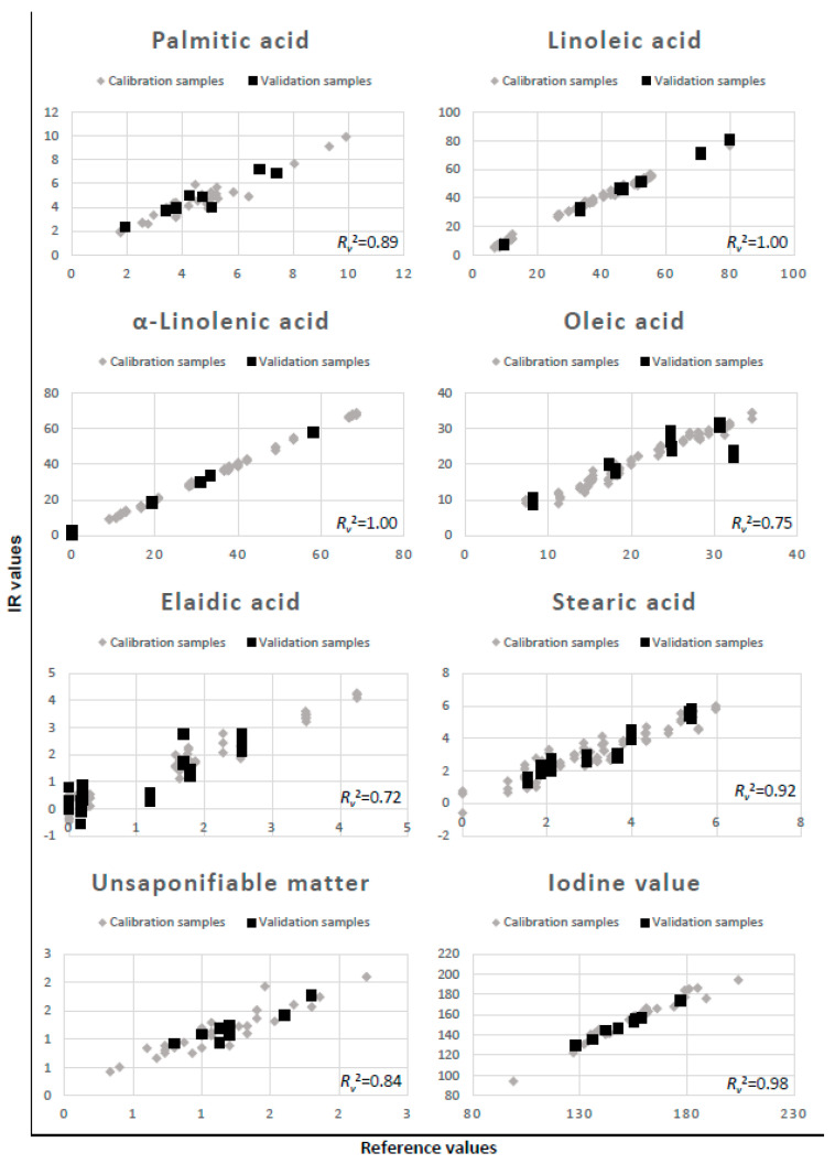
For both the α-linolenic acid and linoleic acid models, R2 of 1.00 was obtained. In the literature models reviewed for these two fatty acids, the content percent was built by Mahboubifar et al. using four types of edible oils and observing the compositional change during heating; for linolenic and linoleic acid, Rv2 was 0.94 and 0.99, respectively [ref. 27]. In this reference, models for palmitic acid, stearic acid, and oleic acid were also built, obtaining Rv2 values of 0.99, 0.97, and 0.98, respectively. In our study, the highest Rv2 values obtained for these fatty acid contents were 0.89, 0.92, and 0.75, respectively.
The highest Rv2 value obtained for iodine value prediction was 0.98. Similarly, other authors have made very good models for iodine value prediction [ref. 25,ref. 34]. Dyminska et al. analyzed 13 different oils (sunflower, avocado, hemp, high-linolenic flax, low-linolenic flax, safflower, walnut, roasted sesame, rice, corn, rapeseed, pumpkin seed, hazel) and obtained a model based on IR spectral data with Rv2 = 0.988. This study used a similarly heterogenic set of different oil types but with a smaller number of samples [ref. 34]. Additionally, Sanchez et al. analyzed the iodine value in hydrogenated soybean oil using FTIR-ATR and built a model for iodine value prediction with Rv2 = 0.987. However, the purpose of this study was very different to ours. Only one type of oil was used, and the aim was to monitor changes in the iodine value during a very specific process: hydrogenation [ref. 25]. In our study, the aim was to control the quality of different types of specific oils not subjected to any deterioration process.
Some variables had very low Rv2 values. Models for the peroxide value had the highest Rv2 value of 0.49. In the reviewed literature, models for peroxide values have Rv2 values ranging between 0.701 and 0.997. Good models for the peroxide value are mostly obtained for a small number of oil types studied, mostly single plant sources, during oxidation processes such as heating or frying [ref. 22,ref. 23,ref. 26,ref. 27]. Molecules containing -OH groups overlap with the hydroperoxide band, which interferes with the determination of the peroxide value. Such molecules are mainly alcohols, phytosterols, mono- and diglycerides, free fatty acids, and water [ref. 23].
We were not able to obtain a good model for the acid value, saponification value, ester value, and hydroxyl value with our methods. In the reviewed literature, we found that Mahboubifar et al. built a model for acid value prediction with Rv2 0.86 [ref. 27]. Similar to the peroxide value, the aim of this study was to monitor the variation in the composition of oil during heating. Bendini et al. built a good model for predicting the acid value for olive oils with Rv2 0.955; compared to our study, their sample set was composed of only one plant-type oil [ref. 23].
In our study, the same process for variable selection was used for all dependent variables. The results showed that this is not suitable for all of them. For the peroxide value, acid value, saponification value, ester value, and hydroxyl value, models can be improved by finding and selecting even more specific parts of the spectra, excluding irrelevant data for these dependent variables.
In Table 4, the FT-IR method is compared to reference methods for vegetable oil characterization. In the FT-IR method, the most time-consuming and difficult part is the method development and validation part. Once the method is developed for a given application, the analysis is fast and easily carried out with little chance of human error. In titration methods, there are many toxic chemicals used and laboratory skills are important for the accuracy and repeatability of analysis. Gas chromatography for fatty acid quantification requires appropriate sample preparation, which again uses toxic organic chemicals. Gas chromatography itself can be automated; however, the analysis is long.
Table 4: Comparison of the FT-IR method and currently used methods for vegetable oil characterization.
| Titration (Acid, Hydroxyl, Iodine, Peroxide, Saponification Value) | Gas Chromatography (Fatty Acid Content) | FT-IR | |
|---|---|---|---|
| Method development | developed | developed | has to be developed and validated |
| Time consumption | long | long | fast |
| Amount of sample | grams | miligrams | miligrams |
| Repeatability | poor | good | good |
| Chemicals | toxic organic | toxic organic | none |
| Ease of analysis | good laboratory skills | good laboratory skills | easy |
| Laboratory equipment | basic | expensive | expensive |
4. Materials and Methods
4.1. Samples
Thirty-seven commercially available vegetable oils used as cosmetic ingredients and as food or food supplements were collected. Among these oils, there were 18 different types of oils and one to four samples for each type of oil. Each type of oil had one or two representatives in the calibration dataset; if there were three or more samples of the same type, the rest were put into the validation set. Validation samples were chosen randomly, excluding minimal or maximal values for each dependent variable where possible. The samples, manufacturer, and type of dataset are presented in Table 5.
Table 5: Samples of vegetable oils used in the analysis.
| Plant of the Oil Source | Latin Name of the Plant | Supplier | Calibration or Validation Dataset |
|---|---|---|---|
| Cranberry seed oil | Vaccinum macrocarpon | Behawe Naturprodukte, Germany | Calibration |
| Cranberry seed oil | Vaccinum macrocarpon | Alexmo Cosmetics, Germany | Calibration |
| Cranberry seed oil | Vaccinum macrocarpon | Dragonspice Naturwaren, Germany | Validation |
| Elderberry seed oil | Sambucus nigra | Baccararose, Germany | Calibration |
| Elderberry seed oil | Sambucus nigra | Behawe Naturprodukte, Germany | Calibration |
| Borage seed oil | Borago officinalis | Dragonspice Naturwaren, Germany | Validation |
| Borage seed oil | Borago officinalis | Tovarna Organika, Slovenia | Validation |
| Borage seed oil | Borago officinalis | Caelo, Germany | Calibration |
| Borage seed oil | Borago officinalis | Farmalabor, Italy | Calibration |
| Blackcurrant seed oil | Ribes nigrum | Dragonspice Naturwaren, Germany | Calibration |
| Blackcurrant seed oil | Ribes nigrum | Behawe Naturprodukte, Germany | Calibration |
| Hemp seed oil | Cannabis sativa | Dragonspice Naturwaren, Germany | Calibration |
| Hemp seed oil | Cannabis sativa | Tovarna Organika, Slovenia | Calibration |
| Hemp seed oil | Cannabis sativa | Manske, Germany | Validation |
| Raspberry seed oil | Rubus idaeus | Tovarna Organika, Slovenia | Validation |
| Raspberry seed oil | Rubus idaeus | Dragonspice Naturwaren, Germany | Calibration |
| Raspberry seed oil | Rubus idaeus | Behawe Naturprodukte, Germany | Calibration |
| Black mustard seed oil | Brassica nigra | Behawe Naturprodukte, Germany | Calibration |
| Walnut seed oil | Juglans regia | Baccararose, Germany | Calibration |
| Walnut seed oil | Juglans regia | Caelo, Germany | Calibration |
| Sea buckthorn seed oil | Hippophae rhamnoides | Dragonspice Naturwaren, Germany | Calibration |
| Sea buckthorn seed oil | Hippophae rhamnoides | Behawe Naturprodukte, Germany | Calibration |
| Evening primrose seed oil | Oenothera biennis | Dragonspice Naturwaren, Germany | Validation |
| Evening primrose seed oil | Oenothera biennis | Farmalabor, Italy | Calibration |
| Evening primrose seed oil | Oenothera biennis | Alexmo Cosmetics, Germany | Calibration |
| Evening primrose seed oil | Oenothera biennis | Caelo, Germany | Validation |
| Rosehip seed oil | Rosa canina | Manske, Germany | Calibration |
| Rosehip seed oil | Rosa canina | Alexmo Cosmetics, Germany | Calibration |
| Chia seed oil | Salvia hispanica | Baccararose, Germany | Calibration |
| Chia seed oil | Salvia hispanica | Dragonspice Naturwaren, Germany | Calibration |
| Perilla seed oil | Perilla frutescens | Baccararose, Germany | Calibration |
| Black cumin seed oil | Nigella sativa | Caelo, Germany | Calibration |
| Sacha inchi seed oil | Plukenetia volubilis | Magnolija, Slovenia | Calibration |
| Kiwi seed oil | Actinidia chinensis | Dragonspice Naturwaren, Germany | Calibration |
| Lineseed oil | Linum usitatissimum | Baccararose, Germany | Validation |
| Lineseed oil | Linum usitatissimum | Farmalabor, Italy | Calibration |
| Lineseed oil | Linum usitatissimum | Caelo, Germany | Calibration |
4.2. Chemical Characterization of Vegetable Oils
The acid value, saponification value, ester value, hydroxyl value (method A), iodine value (method B), peroxide value (method B), and unsaponifiable matter were determined by the procedures described in European Pharmacopoeia 8.0, sections 2.5.1–2.5.7.
4.3. GC–MS Analysis of Fatty Acid Composition
First, the transesterification of fatty acids was carried out to make the constituents volatile for GC–MS analysis. The sample was injected to the GC column for separation of the constituents. They were detected by an MS detector and the identification was carried out by reference compounds and MS spectral libraries.
In situ transesterification was carried out for 10 mg of samples, adding 10 μL of dichloromethane and 200 μL of 0.5 M NaOH in methanol. The mixture was then heated in a water bath at 90 °C for 10 min. After cooling, 200 μL of 14% BF3 in methanol was added, and the mixture was heated again at 90 °C for 10 min. Then, 200 μL of demineralized water and 1 mL of hexane were added and shaken intensively for 1 min for extraction. The hexane phase was analyzed by GC–MS. A gas chromatograph (GCMS-QP2010 Ultra; Shimadzu, Kyoto, Japan) was used to analyze the material. A capillary column was used (Rtx-1 F&F; 30 m × 0.25 mm i.d.; film thickness, 0.25 μm; Restek, Bellefonte, PA, USA). The temperature program began at 160 °C and the temperature was then raised to 250 °C at 3 °C/min. The injection temperature was 250 °C, the temperature of the ion source was 200 °C, and the temperature of the interface was 280 °C. The injection volume was 1 µL, the split ratio was 1:100, the carrier gas was He, and the flow linear velocity was 1 mL/min. The mass spectrometry conditions included electron impact mode at an ionization voltage of 70 eV, with the total ion current recorded, with a scan range from 35 m/z to 500 m/z at a frequency of 5 Hz. The detector voltage was 1 kV. The total analysis time was 30 min. The compounds were identified by comparing their mass spectra and retention indices to the spectra and retention indices of the reference compounds obtained from standard Supelco F.A.M.E. MIX, C4-C24 (Sigma-Aldrich, Steinheim, Germany) and to the spectra and retention indices obtained from the Flavors and Fragrances of Natural and Synthetic Compounds spectral library (FFNSC3) and National Institute of Standards and Technology spectral library (NIST11). Concentrations were calculated as relative peak areas, and fatty acid contents are given in %.
4.4. Recording of the IR Spectra
4.4.1. ATR Spectra
ATR FT-IR spectra were collected using a diamond attenuated total reflection (ATR) accessory from Dura SamplIR Technologies coupled to a Nicolet Instrument Co spectrometer using a DTGS detector. The spectrometer was linked to a computer equipped with Omnic E.S.P. 5.2 software to allow for the automated collection of IR spectra.
Each spectrum was collected as an average of 50 scans between 500 cm−1 and 4000 cm−1. Spectra were collected at three different resolutions: 2 cm−1, 4 cm−1, and 8 cm−1. Three spectra at each resolution were collected for each sample. A new background was collected at each resolution before the three measurements for one sample because of the CO2 peak. For data analysis and model building, all three spectra obtained for one sample were used separately or averaged.
4.4.2. Transmissive Spectra
Transmissive FT-IR spectra were collected using a SpectraTech extension for NaCl plates coupled to a Nicolet Instrument Co spectrometer using a DTGS detector. The spectrometer was linked to a computer equipped with Omnic E.S.P. 5.2 software to allow for the automated collection of IR spectra.
Vegetable oils were diluted in dichloromethane vol/vol = 1/10, and one droplet was placed onto a NaCl plate (11 × 30 × 7 mm) and left alone for dichloromethane to evaporate. The NaCl plate was completely cleaned between different samples with saturated NaCl ethanol solution and only wiped between three consecutive measurements of the same sample. Each spectrum was collected as an average of 50 scans between 600 cm−1 and 4000 cm−1. Spectra were collected at three different resolutions: 2 cm−1 (R2), 4 cm−1 (R4), and 8 cm−1 (R8). Three spectra at each resolution were collected for each sample. A new background was collected at each resolution before the three measurements for one sample because of the CO2 peak. For data analysis and model building, all three spectra obtained for one sample were used separately or averaged.
4.5. Data Analysis
After collecting the infrared spectra, they were first preprocessed with different techniques; in the next step, the important variables were extracted by different methods. Models were then built using partial least squares regression (PLS). In the last step, the validation with an independent set of samples was carried out and parameters to assess the quality of the models were calculated.
Spectral data analyses were carried out using Octave 5.1.0. A total of 7488 models were built for all 13 predictive variables using all possible combinations of the 5 parameters (spectra measurement technique, resolution, separate or averaged spectra, predictive variable selection, and spectra preprocessing). Spectra were measured using ATR and the transmission method. Models were built using three separate spectra for each sample and compared to models built using averaged spectra for each sample. Samples were divided into calibration and validation sets. In cases where three spectra for the same sample were included in the analysis, all three spectra were assigned to the same for the two sets. Spectra were collected at three different resolutions. Different spectra preprocessing techniques were used for all spectra: raw spectra, first and second derivative, normalization (NOR), first and second derivative of normalization, standard normal variate (SNV), first and second derivative of SNV, Haar wavelet transform, and the first and second derivative of data obtained with the Haar wavelet transform. The wavelet transform yields two datasets: the approximate coefficients (WA) and the detailed coefficients (WD), both of which were compared. As there are many variables in the IR spectrum and many statistical processes, we also used random data, which were treated as one of the preprocessing techniques. In this case, the matrix data were filled with random numbers instead of spectral data. The aim was to check that it is not possible to obtain good models with random data.
Spectra contain a large number of variables; different methods were used for lowering the number of these variables to approximately 40% for spectral data before applying the partial least squares (PLS) method. In the first case (CORR), these variables were selected using the Pearson correlation, where 40% of all spectral variables were chosen based on the largest absolute correlation with the dependent variable for which the model was built. Another technique (CHEM) was to first lower the number of spectral variables, taking in the parts of the spectra where absorption peaks for important chemical bonds exist; the selected spectral ranges were 600–1500 cm−1, 1600–1800 cm−1, 2850–3050 cm−1, and 3400–3500 cm−1. The third technique (STD) used for lowering the number of variables involved selecting 40% of spectral variables based on the largest standard deviation. The hypothesis was that where spectra change most among samples, there is important information available for differentiation.
To obtain the most appropriate number of latent factors used in PLS, the leave-one-out method was used for the calibration set to test for the 1–20 latent factors used.
The quality of the models was assessed using the correlation R2 of the calibration (Rc2) and validation (Rv2) sets of samples and the root-mean-square error of calibration (RMSEC), root-mean-square error of validation (RMSEV), and root-mean-square error of prediction (RMSEP).
5. Conclusions
The methods used give good models for predicting the content of the fatty acids studied, while good models for predicting pharmacopoeia chemical values are obtained only for iodine value and unsaponifiable matter. For some variables, such as the linoleic and α-linolenic acid content and iodine number, a large number of good models are obtained. In this case, the method of spectral recording, selection, and processing of spectral variables is not very important. For the other variables, good models are obtained only with the appropriate choice of recording and processing of spectral data. Based on our results, we conclude that infrared spectroscopy offers a good supplemental or alternative method for the determination of vegetable oil quality.
References
- D.D. Wang, F.B. Hu. Dietary Fat and Risk of Cardiovascular Disease: Recent Controversies and Advances. Annu. Rev. Nutr., 2017. [DOI | PubMed]
- A. Locke, J. Schneiderhan, S.M. Zick. Diets for Health: Goals and Guidelines. Am. Fam. Physician, 2018. [PubMed]
- N. Poljšak, S. Kreft, N. Kočevar Glavač. Vegetable Butters and Oils in Skin Wound Healing: Scientific Evidence for New Opportunities in Dermatology. Phytother. Res., 2020. [DOI | PubMed]
- A.R. Vaughn, A.K. Clark, R.K. Sivamani, V.Y. Shi. Natural Oils for Skin-Barrier Repair: Ancient Compounds Now Backed by Modern Science. Am. J. Clin. Dermatol., 2018. [DOI | PubMed]
- Y.A. Negash, D.E. Amare, B.D. Bitew, H. Dagne. Assessment of Quality of Edible Vegetable Oils Accessed in Gondar City, Northwest Ethiopia. BMC Res. Notes, 2019. [DOI | PubMed]
- R. Ganguly, G.N. Pierce. The Toxicity of Dietary Trans Fats. Food Chem. Toxicol., 2015. [DOI | PubMed]
- P. Perjesi, Z. Pinter, Z. Gyongyi, I. Ember. Effect of Rancid Corn Oil on Some Onco/Suppressor Gene Expressions in Vivo. A Short-Term Study-PubMed. Anticancer Res., 2002. [PubMed]
- 8.European Pharmacopoeia (Ph. Eur.)8th ed.EDQM-European Directorate for the Quality of MedicinesStrasbourg, France2013
- C.W. Kwon, K.M. Park, J.W. Park, J. Lee, S.J. Choi, P.S. Chang. Rapid and Sensitive Determination of Lipid Oxidation Using the Reagent Kit Based on Spectrophotometry (FOODLAB Fat System). J. Chem., 2016. [DOI]
- W.E. Gilbraith, J.C. Carter, K.L. Adams, K.S. Booksh, J.M. Ottaway. Improving Prediction of Peroxide Value of Edible Oils Using Regularized Regression Models. Molecules, 2021. [DOI | PubMed]
- E.I. Geana, C.T. Ciucure, C. Apetrei, V. Artem. Application of Spectroscopic UV-Vis and FT-IR Screening Techniques Coupled with Multivariate Statistical Analysis for Red Wine Authentication: Varietal and Vintage Year Discrimination. Molecules, 2019. [DOI]
- Z. Wu, Y. Zhao, J. Zhang, Y. Wang. Quality Assessment of Gentiana Rigescens from Different Geographical Origins Using FT-IR Spectroscopy Combined with HPLC. Molecules, 2017. [DOI | PubMed]
- G.O. Ildiz, A. Karadag, E. Kaygisiz, R. Fausto. PLS-DA Model for the Evaluation of Attention Deficit and Hyperactivity Disorder in Children and Adolescents through Blood Serum FTIR Spectra. Molecules, 2021. [DOI | PubMed]
- J. Luypaert, M.H. Zhang, D.L. Massart. Feasibility Study for the Use of near Infrared Spectroscopy in the Qualitative and Quantitative Analysis of Green Tea, Camellia Sinensis (L.). Anal. Chim. Acta, 2003. [DOI]
- M. Kokalj, M. Rihtarič, S. Kreft. Commonly Applied Smoothing of IR Spectra Showed Unappropriate for the Identification of Plant Leaf Samples. Chemom. Intell. Lab. Syst., 2011. [DOI]
- E. Junaedi, K. Lestari, M. Muchtaridi. Infrared Spectroscopy Technique for Quantification of Compounds in Plant-Based Medicine and Supplement. J. Adv. Pharm. Technol. Res., 2021. [PubMed]
- P. Geladi, H. Martens, L. Hadjiiski, P. Hopke. A Calibration Tutorial for Spectral Data. Part 2. Partial Least Squares Regression Using Matlab and Some Neural Network Results. J. Near Infrared Spectrosc., 1996. [DOI]
- M. Kokalj, S. Strgulc Krajšek, J. Omahen Bratuša, S. Kreft. Comparison and Improvement of Commonly Applied Statistical Approaches for Identification of Plant Species from IR Spectra. J. Chemom., 2010. [DOI]
- D. Guille, N. Cabo. Infrared Spectroscopy in the Study of Edible Oils and Fats. J. Sci. Food Agric., 1997. [DOI]
- N. Vlachos, Y. Skopelitis, M. Psaroudaki, V. Konstantinidou, A. Chatzilazarou, E. Tegou. Applications of Fourier Transform-Infrared Spectroscopy to Edible Oils. Anal. Chim. Acta, 2006. [DOI]
- Q. Zhang, C. Liu, Z. Sun, X. Hu, Q. Shen, J. Wu. Authentication of Edible Vegetable Oils Adulterated with Used Frying Oil by Fourier Transform Infrared Spectroscopy. Food Chem., 2012. [DOI | PubMed]
- P. Liang, C. Chen, S. Zhao, F. Ge, D. Liu, B. Liu, Q. Fan, B. Han, X. Xiong. Application of Fourier Transform Infrared Spectroscopy for the Oxidation and Peroxide Value Evaluation in Virgin Walnut Oil. J. Spectrosc., 2013. [DOI]
- A. Bendini, L. Cerretani, F. DI Virgilio, P. Belloni, M. Bonoli-Carbognin, G. Lercker. Preliminary evaluation of the application of the ftir spectroscopy to control the geographic origin and quality of virgin olive oils. J. Food Qual., 2007. [DOI]
- F.R. van de Voort, A.A. Ismail, J. Sedman, J. Dubois, T. Nicodemo. The Determination of Peroxide Value by Fourier Transform Infrared Spectroscopy. J. Am. Oil Chem. Soc., 1994. [DOI]
- J.L. Sanchez, S.B.G. Pereira, P.C. de Lima, G. Possebon, A. Tanamati, R.J. Poppi, A.A.C. Tanamati, E. Bona. Mid-Infrared Spectroscopy and Support Vector Machines Applied to Control the Hydrogenation Process of Soybean Oil. Eur. Food Res. Technol., 2017. [DOI]
- S. Tinggi Farmasi Borneo Lestari, S. Kalimantan. Determination of Peroxide Value of Red Fruit Oil by FTIR Spectroscopy and Multivariate Calibration. Int. Food Res. J., 2017
- M. Mahboubifar, S. Yousefinejad, M. Alizadeh, B. Hemmateenejad. Prediction of the Acid Value, Peroxide Value and the Percentage of Some Fatty Acids in Edible Oils during Long Heating Time by Chemometrics Analysis of FTIR-ATR Spectra. J. Iran. Chem. Soc., 2016. [DOI]
- K. Wójcicki, I. Khmelinskii, M. Sikorski, E. Sikorska. Near and Mid Infrared Spectroscopy and Multivariate Data Analysis in Studies of Oxidation of Edible Oils. Food Chem., 2015. [DOI | PubMed]
- J.Y. Chen, H. Zhang, J. Ma, T. Tuchiya, Y. Miao. Determination of the Degree of Degradation of Frying Rapeseed Oil Using Fourier-Transform Infrared Spectroscopy Combined with Partial Least-Squares Regression. Int. J. Anal. Chem., 2015. [DOI | PubMed]
- H. Zhang, J. Ma, Y. Miao, T. Tuchiya, J.Y. Chen. Analysis of Carbonyl Value of Frying Oil by Fourier Transform Infrared Spectroscopy. J. Oleo Sci., 2015. [DOI | PubMed]
- C. Pizarro, I. Esteban-Díez, S. Rodríguez-Tecedor, J.M. González-Sáiz. Determination of the Peroxide Value in Extra Virgin Olive Oils through the Application of the Stepwise Orthogonalisation of Predictors to Mid-Infrared Spectra. Food Control, 2013. [DOI]
- A.S. Luna, A.P. Da Silva, J. Ferré, R. Boqué. Classification of Edible Oils and Modeling of Their Physico-Chemical Properties by Chemometric Methods Using Mid-IR Spectroscopy. Spectrochim. Acta Part A Mol. Biomol. Spectrosc., 2013. [DOI | PubMed]
- F.R. van de Voort, A.A. Ismail, J. Sedman, G. Emo. Monitoring the Oxidation of Edible Oils by Fourier Transform Infrared Spectroscopy. J. Am. Oil Chem. Soc., 1994. [DOI]
- L. Dymińska, M. Calik, A.M.M. Albegar, A. Zając, K. Kostyń, J. Lorenc, J. Hanuza. Quantitative Determination of the Iodine Values of Unsaturated Plant Oils Using Infrared and Raman Spectroscopy Methods. Int. J. Food Prop., 2017. [DOI]