Domesticated cannabinoid synthases amid a wild mosaic cannabis pangenome

Article type: Research Article

Keywords: Molecular evolution, Transposition, Plant evolution, Natural variation in plants, Plant breeding

Authors: Ryan C. Lynch ⚬, Lillian K. Padgitt-Cobb ⚬, Andrea R. Garfinkel, Brian J. Knaus ⚬, Nolan T. Hartwick, Nicholas Allsing ⚬, Anthony Aylward, Philip C. Bentz ⚬, Sarah B. Carey ⚬, Allen Mamerto, Justine K. Kitony, Kelly Colt ⚬, Emily R. Murray ⚬, Tiffany Duong, Heidi I. Chen ⚬, Aaron Trippe ⚬, Alex Harkess ⚬, Seth Crawford, Kelly Vining, Todd P. Michael ⚬

Affiliations: https://ror.org/03xez1567grid.250671.70000 0001 0662 7144The Plant Molecular and Cellular Biology Laboratory, The Salk Institute for Biological Studies, La Jolla, CA USA; Oregon CBD, Independence, OR USA; https://ror.org/00ysfqy60grid.4391.f0000 0001 2112 1969Department of Horticulture, Oregon State University, Corvallis, OR USA; https://ror.org/04nz0wq19grid.417691.c0000 0004 0408 3720HudsonAlpha Institute for Biotechnology, Huntsville, AL USA; https://ror.org/0168r3w48grid.266100.30000 0001 2107 4242Department of Cell and Developmental Biology, School of Biological Sciences, University of California San Diego, La Jolla, CA USA; Science and Conservation, San Diego Botanical Garden, Encinitas, CA USA; https://ror.org/0168r3w48grid.266100.30000 0001 2107 4242Center for Marine Biotechnology and Biomedicine, University of California San Diego, La Jolla, CA USA

License: © The Author(s) 2025 CC BY 4.0 Open Access This article is licensed under a Creative Commons Attribution 4.0 International License, which permits use, sharing, adaptation, distribution and reproduction in any medium or format, as long as you give appropriate credit to the original author(s) and the source, provide a link to the Creative Commons licence, and indicate if changes were made. The images or other third party material in this article are included in the article’s Creative Commons licence, unless indicated otherwise in a credit line to the material. If material is not included in the article’s Creative Commons licence and your intended use is not permitted by statutory regulation or exceeds the permitted use, you will need to obtain permission directly from the copyright holder. To view a copy of this licence, visit http://creativecommons.org/licenses/by/4.0/.

Article links: DOI: 10.1038/s41586-025-09065-0  |  PubMed: 40437092  |  PMC: PMC12286863

Relevance: Relevant: mentioned in keywords or abstract

Full text: PDF (1.6 MB)

Main

Cannabis (C. sativa L., cannabis) is an ancient domesticated plant with widespread archaeological evidence for seed (achene) and fibre utilization dating to 8,000 years ago in East Asia, and earlier occurrences found up to 12,000 years ago^1,2, rivalling that of important crops such as wheat, barley, maize and rice. Cannabis was originally a multipurpose crop in Asia, where the same plants were utilized as a source of fibre, food and drugs^2,3. Over time, cannabis spread globally and single or dual-use-type cultivars were developed, eventually giving rise to divergent hemp and drug-type populations of the twentieth century⁴. Prior to the early 1900s, cannabis was an important commodity across Asia, Europe and the New World, and was used to produce fibres used in sails, ropes, clothing and paper. However, competition from other fibre crops, entanglement with drug laws, and the eventual development of synthetic fibres led to a decline in production. In recent decades, the use of cannabis has shifted to specialized applications, including niche seed oils and drug production, where it continues to hold significant economic and cultural importance today⁵.

Throughout history and around the world, cannabis has undergone cycles of “cultivation, consumption, and crackdown”⁶. Modern prohibition originated in the USA during the early twentieth century⁷, but by 1961 had spread to a majority of countries⁸. Prohibition eliminated the fibre and food uses of cannabis for decades, but gave rise to a high-value illegal market for phytocannabinoid-based drugs, which are derived from glandular trichomes. Although more than 100 phytocannabinoids have been identified, only a limited number are produced in significant quantities, which are used to classify plants by chemotype: delta-9-tetrahydrocannabinolic acid (THCA; type I), cannabidiolic acid (CBDA; type III), balanced CBDA and THCA (type II), cannabigerolic acid (CBGA; type IV) and cannabinoid-free (type V)⁹. Although tetrahydrocannabinol (THC), the primary intoxicant, remains a controlled substance, a majority of US states and many countries now allow medical or adult use of cannabis products. Separately, the 2014 and 2018 US Farm Bills facilitated hemp production and research in plants that produce less than 0.3% THC on US soil, generating opportunities for improved non-THC drug, grain and fibre applications.

The haploid cannabis genome is relatively small in size (around 750 Mb), yet its complexity is driven by a high proportion (approximately 79%) of transposable elements (TEs) and substantial heterozygosity (single nucleotide polymorphisms (SNPs): greater than 2%). The CBDRx (cs10) reference genome, derived from the high-cannabinoid (HC) cannabidiol (CBD) hemp lineage related to the well-known anti-epileptic ‘Charlotte’s web’ cultivar¹⁰, resolved the arrangement of cannabinoid synthase genes as a single full-length copy of CBDAS nested within conserved 70 to 80-kb tandem TE arrays. Furthermore, HC hemp lines such as CBDRx emerged through the introgression of the CBDAS locus into a predominantly marijuana (MJ) genetic background, thereby leveraging high-potency alleles to enhance CBD production¹¹. However, initial comparison of published cannabis genomes suggests substantial genomic dynamism across use types^11–16, raising key unresolved questions about the global extent of genetic diversity. Additionally, the role of hybridization in shaping genome architecture and allele transmission remains unclear, highlighting the need for further high-quality assemblies and population-scale genomic analyses. Here we have built a comprehensive framework for exploring genetic diversity in this multi-use crop by creating a cannabis pangenome using haplotype-resolved, chromosome-scale assemblies.

The cannabis pangenome

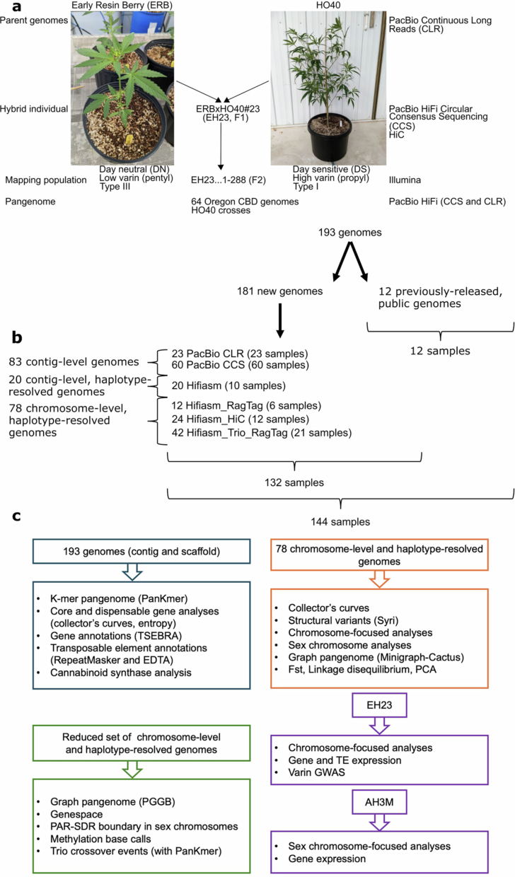
Cannabis is often classified as a monospecific genus¹⁷, although debate remains regarding the status of Cannabis indica Lam. and Cannabis ruderalis, the latter of which is thought to be the source of the day-neutral (DN; autoflowering) flowering type¹⁸. We addressed the diversity of cannabis by building the pangenome with samples selected from multiple sources to cover use types, history, sex expression and agronomic traits (Extended Data Fig. 1 and Supplementary Fig. 1). The cannabis pangenome comprises 181 new PacBio assemblies and 12 previously published genomes, representing 144 biological samples, including 78 haplotype-resolved, chromosome-scale assemblies and 103 contig-level assemblies. We highlight an F₁ hybrid (ERBxHO40_23; EH23) between two phenotypically and genetically divergent parents to clarify features of the genome that have been missed in previous studies (Fig. 1a, Extended Data Figs. 2 and 3 and Supplementary Note 1).

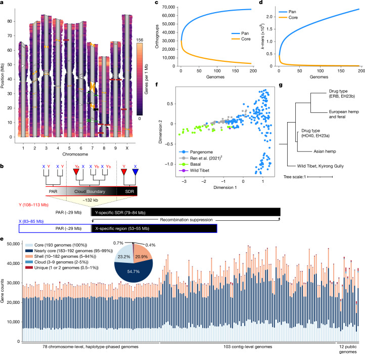
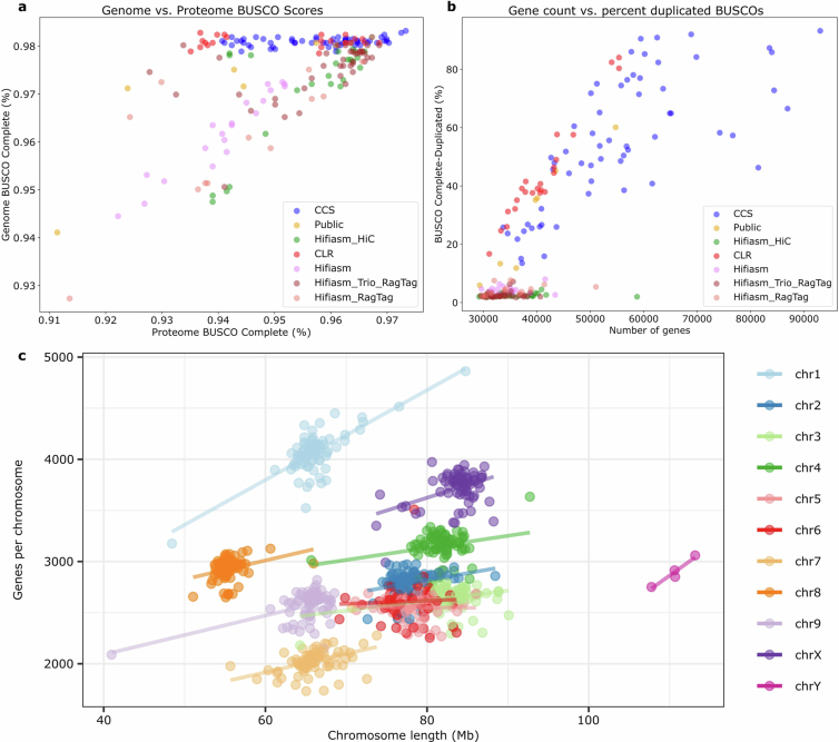
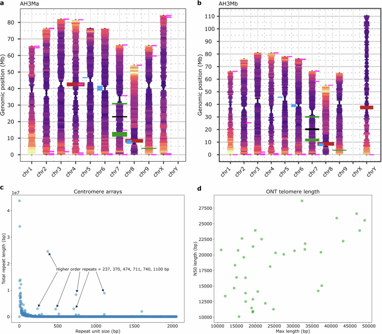
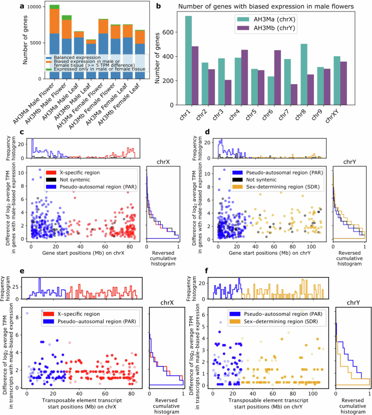
All genomes are of high quality, with an average N50 of 7.5 Mb, and BUSCO¹⁹ genome and proteome completeness scores of 97% and 95%, respectively (Extended Data Fig. 4). The average haploid genome length was 781 Mb with around 35,000 protein-coding genes per genome (Supplementary Tables 1, 2 and 3). Consistent with a predominantly outcrossing behaviour, the SNP-based heterozygosity ranged between 1% and 2.5% (Supplementary Fig. 2). The assemblies are also high quality structurally, resolving previous TE placement issues (Supplementary Fig. 3) and revealing centromere regions, telomere length, large structural variations (SVs), fine-scale genetic architecture of important genes such as the cannabinoid synthases, as well as the sex-determining region (SDR) and pseudoautosomal region (PAR) of the Y chromosome (Fig. 1a,b), the largest chromosome in the Cannabis genome (Extended Data Fig. 5).

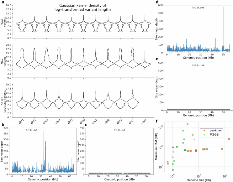
We constructed comprehensive Cannabis pangenomes using both reference-based and reference-free approaches. A reference-based pangenome graph was generated with Minigraph-Cactus (MGC)²⁰ using the 78 chromosome-scale, haplotype-resolved genomes. For a reference-free approach, we built a k-mer matrix with PanKmer²¹ using all 193 genomes and a graph-based representation with PanGenome Graph Builder (PGGB)²². Owing to the high memory demands of PGGB, we selected a subset of 16 genomes for graph generation (Extended Data Fig. 6 and Methods). SVs detected by MGC and PGGB closely matched those from pairwise whole-genome alignments. Mapping rates for a diverse short-read dataset² were similar between the MGC pangenome graph (95.09%) and the linear EH23a reference genome (95.0%), indicating that both approaches effectively captured variation.

The pangenome reveals five populations

The taxonomy, history and nomenclature of the cannabis genus have long been debated²³. Owing to its wide phenotypic and geographic diversity, it has been classified either as a multi-species interbreeding complex or as a single species with subspecies designations. We calculated the collector’s curve to evaluate the completeness and diversity of the pangenome using shared gene-based orthogroups as well as shared k-mers (Fig. 1c,d). The curve suggested that we captured the majority of cannabis orthogroup diversity at around 100–125 genomes (Fig. 1c), although significant global genomic variation remains uncharacterized (Fig. 1d), possibly owing to the recent TE activity. Collector’s curves for the 78 haplotype-resolved, chromosome-scale assemblies revealed similar but more attenuated diversity–sample relationships (Supplementary Fig. 4). Across all pangenome samples we found that 23% of genes were ‘core’ (present in all genomes), 55% were ‘nearly-core’ (95–99% of genomes), 21% were ‘shell’ (5–94% of genomes), and a small fraction were classified as ‘cloud’ (0.4%) or ‘unique’ (0.7%) (Fig. 1e and Supplementary Fig. 5). Gene Ontology (GO) terms related to terpene biosynthesis and defence response were some of the most frequently enriched among core genes (Extended Data Fig. 7, Supplementary Note 2 and Supplementary Table 4), although both showed substantial variation at the sequence level (Extended Data Figs. 7 and 8).

Cannabis has not undergone a whole-genome duplication since the ancient lambda event approximately 100 million years ago¹³. This suggests that its extensive genomic diversity arose not through recent whole-genome duplications or hybridization-driven allopolyploidy, but through tandem gene duplication and other local duplication mechanisms (Supplementary Fig. 6 and Supplementary Note 3). Comparisons between populations using pairwise average F_st (fixation index) values based on phased SNPs indicated that some cannabis populations exhibited levels of genetic differentiation that were similar to interspecies comparisons, such as in strawberry²⁴ (F_st = 0.20 for MJ versus hemp; Supplementary Table 5). Specific genes with high F_st SNPs were linked to environmental response, with circadian, light signalling and flowering time genes exhibiting an above-average F_st (0.42) (Supplementary Table 6). Notably, GIGANTEA (GI)²⁵, a highly conserved, typically single-copy gene that has a central role in the circadian clock that regulates daily period length, flowering time and cell elongation, contained a SNP with the fifth-highest F_st (0.77, MJ versus hemp). Separately, using a test for selective sweeps across 20-kb SNP windows (XP-CLR, MJ versus hemp), GI was again found within a significant region of the X chromosome. Finally, a broader analysis of gene family diversity revealed substantial variation at the GI locus between the HC hemp and hemp populations (Supplementary Fig. 7). These findings highlight the effect of selection on key agronomic genes²⁶ that may underlie differentiation of traits such as flowering and internode elongation (fibre length), which contrast markedly between hemp and MJ populations.

Drug-type populations from North America that produce high levels of cannabinoids are thought to have originated from regions of Southeast and Central Asia, and were brought to the western hemisphere via the Caribbean and South America; however, most of what is known about these ancestral populations is based on limited historical accounts and speculation⁵. A broad split of drug-type samples into two groups, one aligned with Asian hemp and one with European hemp, was suggested by the k-mer-based hierarchical clustering using the PanKmer pangenome (Fig. 1f,g and Extended Data Fig. 1). Both groups contained MJ and HC hemp samples, which were thought to have largely MJ ancestry with a recent history of introgression breeding for CBDAS genes, perhaps from European hemp origins¹¹. However, using a phased SNP-based structure with all MJ samples treated as a single population, the TreeMix model inferred a highest-likelihood phylogeny that included six gene flow (migration) events between Asian hemp, HC hemp and European hemp, as well as MJ and HC hemp samples (Supplementary Fig. 8). These results may partially explain the European and Asian groupings of drug-type samples found by our k-mer clustering analysis, and reflect the effects of historical hybridization breeding between Asian and European hemp that is documented in the breeding literature²⁷. In addition to the two drug-type populations and separate European and Asian hemp populations, the k-mer clustering showed significant divergence between the single available wild Tibetan assembly from all other domesticated and feral lines,¹³ suggesting that wild Cannabis relatives still exist in remote regions of Asia². Indeed, k-mer based hierarchical clustering of the pangenome assemblies combined with short reads from samples collected across Europe and Asia recapitulated the original authors’ finding that samples from Asia described as ‘drug-type feral’ and ‘basal’ represent distinct populations² (Fig. 1f and Supplementary Fig. 9). Ultimately, refining hypotheses about domestication, biogeography and use-type history will require broader sampling of Asian and historical specimens, along with careful delineation of wild and feral populations.

Sex chromosome evolution

Sex expression in cannabis has long puzzled biologists²⁸. Although most populations are dioecious, with separate male (XY) and female (XX) plants, monoecious (XX) forms also exist, which exhibit variable ratios of male and female flowers. The Cannabaceae sex chromosomes originated in a common ancestor of Cannabis and Humulus more than 36 million years ago (Ma)²⁹—earlier than previous estimates³⁰—making them among the oldest known in flowering plants³¹. Despite their ancient origin, cannabis sex chromosomes have been shaped by human selection on sexually dimorphic traits³². In drug-type populations, males produce few glandular trichomes, and pollination reduces cannabinoid yield in female plants, leading to reduced use (or elimination) of males in breeding programmes (Methods). By contrast, hemp seed production requires pollen, and male plants enhance bast fibre yield and quality. Additionally, European monoecious fibre cultivars, such as Santhica (SAN) and KC Dora (KCDv1), were developed to improve mechanized harvesting efficiency of both fibre and seeds, adding another layer of artificial selection³¹.

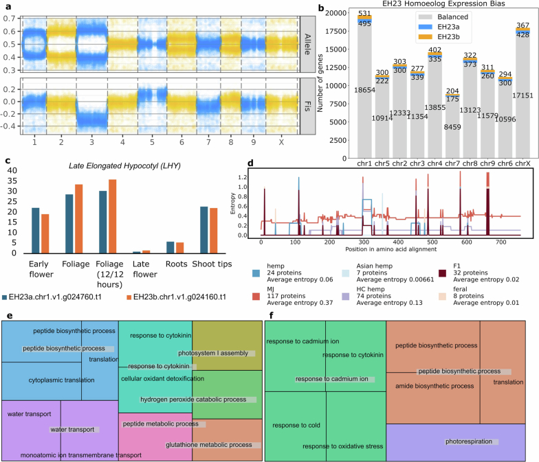
Unlike most angiosperms, cannabis has a heteromorphic XY pair, with a Y chromosome that is approximately 30% larger than the X chromosome (Fig. 1b, Extended Data Figs. 4 and 5). Recombination occurs in the PAR but is suppressed throughout the SDR on the Y chromosome. The SDR spans 79–84 Mb out of the approximately 110 Mb Y chromosome, making it one of the largest SDRs in plants, with 840–1,160 genes (Supplementary Figs. 10 and 11 and Supplementary Tables 7 and 8). By contrast, the PAR covers only around 29 Mb, yet hosts 1,900–1,980 genes, including many important flowering genes, such as FLOWERING LOCUS T (FT), CONSTANS (CO) and GI. Theory predicts that after initial recombination suppression, the SDR expands in a stepwise manner owing to selection linking genes to the SDR that are beneficial to males but deleterious to females³³. Alternatively, neutral processes, reflected in synonymous substitution rates (K_s), can drive SDR expansions. K_s values along the SDR showed a continuous pattern of gene addition from the PAR boundary to the centromere²⁹, suggesting that recombination suppression near the centromere at least partially caused expansion. Using k-mers and X–Y orthologue phylogenies, we identified two distinct SDR haplotypes: Ya, shared by six samples, and Yb, found in two samples (Fig. 1b). These haplotypes differed at the SDR–PAR boundary, separated by 5 conserved gene models spanning approximately 51 kb (GVA-21-1003-002)³⁴ to 132 kb (Kompolti), with all others spanning 61–62 kb. The gene located nearest to the PAR–SDR boundary in the Ya haplotype (within the PAR in Yb; Fig. 1b) is TRANSCRIPTION ELONGATION FACTOR (SPT5), which is known to interact with FLOWERING LOCUS C (FLC) via FRIGIDA during cold-induced flowering in Arabidopsis³⁵. This suggests that selection on flowering time genes has facilitated a stepwise shift in recombination suppression and SDR expansion, which may explain why male flower development begins before female flowering onset in some varieties. Polymorphisms in the SDR–PAR boundary signal that the hemp gene pool hosts ancestral diversity of sexually antagonistic genes, which may underlie useful variation in flowering timing³⁶.

Furthermore, gene expression profiling of Ace High (AH3M) male and female tissue found biased expression of more than 7,000 genes in male flowers across all chromosomes, spanning many functions including pollen development. This contrasted with biased expression of genes in male leaf (approximately 1,400 genes), female leaf (approximately 3,700 genes) and female flower (approximately 3,900 genes) tissue (Extended Data Fig. 9). Whereas gene expression in the X chromosome was fairly uniform, gene density and expression in the Y chromosome were skewed toward the PAR. Of note, a substantial proportion of genes in the PAR (38%, around 750 genes) showed biased expression in male flowers, compared with only 6% (94 genes) in the SDR. Although the SDR encodes one or more unidentified sex-determining genes for male flower development, the majority of the required transcriptional network for male or female flower expression is broadly distributed across all chromosomes.

TEs shape the pangenome

TEs had a major role in shaping the cannabis genome, particularly in the proliferation of intronless cannabinoid synthase genes, which are embedded within 70–80-kb conserved TE cassettes¹¹. On average, TEs comprised 68% of each genome, with long terminal repeat retrotransposons (LTR-RTs) representing 50% of the total (Fig. 2a and Supplementary Tables 1 and 9). Genes on average were located near TEs (443–613 bp from TEs; Supplementary Table 10). Different TE types showed distinct insertion patterns: DNA transposons (for example, Mutator and Helitron) were inserted within 500 bp upstream of coding regions, whereas LTR-RTs were more evenly distributed flanking genes (Supplementary Fig. 12). Genes involved in transposition, transcription, recombination and DNA repair were frequently associated with Ty3-long terminal repeats (LTRs), whereas defence and metabolite biosynthesis genes were enriched near Ty1-LTRs (Supplementary Table 11). Many intact TEs were estimated to have inserted into the genome within the past 100,000 years, suggesting that ongoing diversification may be driven by hybridization and stress factors, particularly in F₁ and MJ populations (Fig. 2a–c). One such factor is clonal propagation, which is a common practice in modern MJ production but is rarely used in hemp field cultivation.

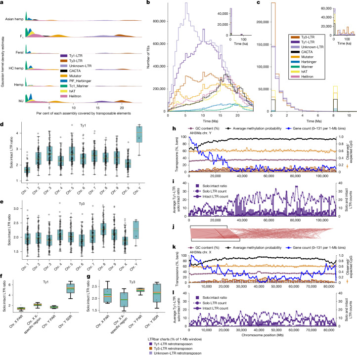
Despite 4 million years of sustained activity and a recent burst of LTR proliferation (Fig. 2b,c), the cannabis genome has maintained a smaller haploid genome size (approximately 750 Mb) than that of its sister genus Humulus, which ranges from 1,700 Mb in Humulus japonicus to 2,700 Mb in Humulus lupulus³⁷. Solo LTRs reflect genome purging and can be formed by ectopic recombination, which occurs in the internal sequence of a complete LTR-RT³⁸. The high solo:intact ratio observed in cannabis (Fig. 2d–g) is likely to contribute to its compact genome size by mitigating TE accumulation. Ty1-LTRs displayed the highest solo:intact ratio within the SDR of the Y chromosome (Fig. 2d,f), suggesting the initial expansion of this region was driven by TE insertions that preceded deletion events by ectopic recombination (Fig. 2i,j). DNA methylation also prevents uncontrolled TE proliferation by silencing expression³⁹. We found that TE methylation levels were higher than genome-wide averages, although population-specific differences were detected (Supplementary Fig. 13 and Supplementary Table 12). We detected expressed TE transcripts in the EH23 F₁ hybrid, indicating ongoing TE activity (Supplementary Fig. 14). On the Y chromosome, the PAR and the SDR exhibited distinct patterns of gene expression and intact TE expression (Extended Data Fig. 9d,f), with the SDR showing increased methylation levels (Fig. 2h), consistent with its degenerate, gene-poor nature. Several TE families are actively transcribed, and many insertions are evolutionarily recent; however, TE frequency profiles varied distinctly among populations (Supplementary Figs. 15 and 16). The combination of recent divergence times for certain TE types (Fig. 2b,c), their enrichment near genes, and their population-specific distributions suggests that TEs contribute to both gene evolution and the regulation of adaptive responses in cannabis.

SVs drive innovation

Given the high abundance of young, active TEs in cannabis, we examined their role in shaping pangenome SVs (Fig. 3). SV counts varied most in translocations and duplications, mirroring population-specific TE abundance (Fig. 2a), whereas inversions showed the least variation (86 per genome on average) (Fig. 3a and Extended Data Fig. 10). However, inversion sizes ranged from 200 bp to 25 Mb (average 304 kb), forming a multi-modal distribution, suggesting that multiple evolutionary forces shaped inversions of different lengths. Whereas the SNP heterozygosity ranged between 1 and 2.5% in the pangenome, the heterozygosity (variable regions) when including SVs and non-alignable regions was on average 20.6% of total genome length (Supplementary Fig. 17), highlighting the extent of previously uncharacterized genomic variation in cannabis.

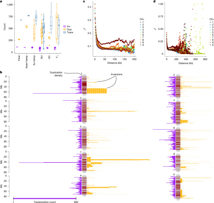
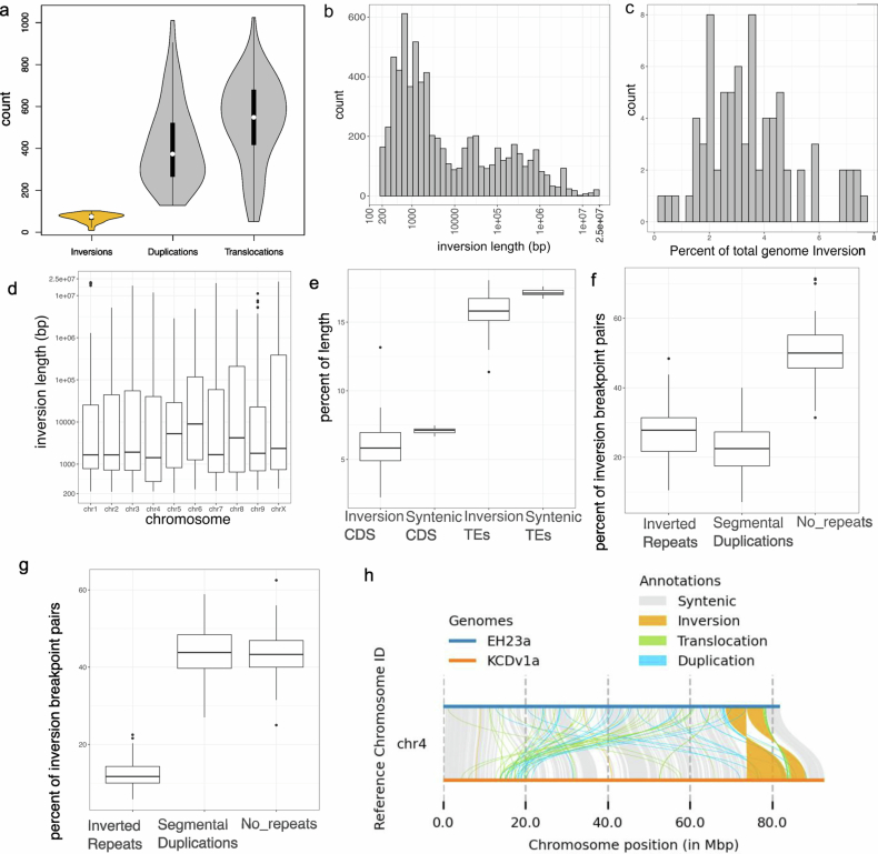
TEs frequently caused small-to-medium translocations, duplications and inversions, whereas larger inversions arose at breakpoints that were enriched with segmental duplications and inverted repeats⁴⁰ (Extended Data Fig. 10). SV hotspots on chromosome (chr.) 1, chr. 4 and chr. 7 overlapped common inversion breakpoints and TE-enriched regions (Fig. 3b). Analysis of TEs within SV breakpoints (500 bp upstream and downstream, 1 kb total) revealed population-specific TE enrichment patterns. In MJ genomes, duplications frequently contained three DNA TE families and Ty3-LTR-RTs (Supplementary Table 13; P < 0.05, Welch’s t-test). Only Harbinger and Mutator DNA TEs were enriched at duplication breakpoints in other populations, whereas feral hemp duplications showed no significant TE enrichment, suggesting recent TE activity or alternative SV formation mechanisms. Inversions covered up to 7% of the genome, surpassing values observed in multi-species comparisons, such as soybean and grapevine⁴¹. Given the population-specific interplay of TEs and SVs, as well as their frequent proximity to genes, our findings revealed a diverse set of mechanisms driving cannabis genome evolution, many of which were undetected in previous resequencing efforts.

Segregation distortion has been observed across multiple regions of the cannabis genome¹⁶, mirroring patterns detected in the F₁ EH23 hybrid (Extended Data Fig. 3), which suggests that SVs may contribute to allele transmission biases⁴². Long inversions, such as the one found on chr. 1 (19.5 Mb in length; Fig. 3b), may function as a supergene, perhaps maintained as a balanced polymorphism through associative overdominance⁴³. Indeed, the 17 instances of this inversion were found to be heterozygous in 15 samples and homozygous in 1. This inverted region contained around 1,203 genes, spanning many functions, including the core circadian and flowering time gene PSEUDO RESPONSE REGULATOR 3 (PRR3), which has been implicated in the ‘autoflower’ DN behaviour in cannabis⁴⁴ as well as in flowering time variation associated with range expansion in major crops (soybean and sorghum) and natural populations^45–47. PRR3 contained a high-F_st SNP (0.61) as well as biased expression in our F₁ EH23 hybrid that was recessive for the DN trait (Extended Data Fig. 3). We found that pairwise SNP r² values and local principal component analysis (PCA) plots of this area suggested some level of haplotype formation and increased linkage disequilibrium (LD; >10 kb) across this region, especially at the interior breakpoint (Fig. 3c,d and Supplementary Fig. 18). However, these were not obvious signals of complete differentiation or recombination suppression as has been shown in other species⁴⁸.

Domesticated cannabinoid pathway

Cannabis is the only prolific producer of cannabinoids, although other plants (such as liverworts) and fungi synthesize smaller quantities⁴⁹. Although key enzymes in the cannabinoid biosynthetic pathway have been identified (Fig. 4a and Supplementary Fig. 19), the genomic organization of the final step in this pathway remained unresolved owing to the complexities of the cannabis genome (Supplementary Fig. 20). This mystery was clarified with the discovery of full-length THCAS, CBDAS and CBCAS genes nested within conserved TE cassettes, arranged in arrays on chr. 7¹¹. However, it was unclear whether this TE-mediated arrangement of synthase genes was conserved across the cannabis pangenome.

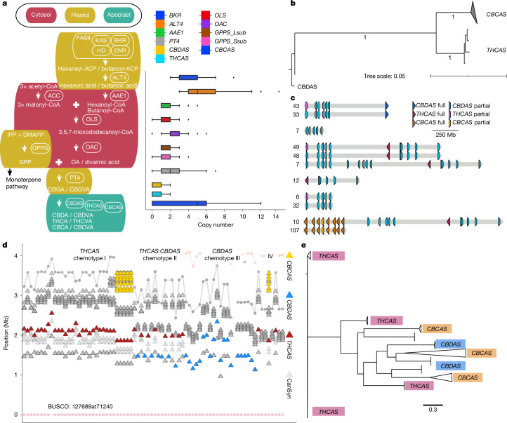
Cannabinoid synthases duplicated and neofunctionalized from the ancestral Berberine bridge enzyme-like (BBE-like) family of genes on chr. 7, then were ultimately reduced to a limited set of functional THCAS and CBDAS alleles through the domestication process^11,50 (Fig. 4b,c and Supplementary Fig. 21). Across the pangenome, each haploid genome hosted a maximum of one full-length THCAS or CBDAS, which were arranged in similar arrays of TE cassettes, most of which contained synthase pseudogenes. These cannabinoid synthase cassettes were found in a limited number of arrangements with association to specific TEs (Fig. 4c,e, Supplementary Figs. 22 and 23 and Supplementary Table 14), which suggested that selection had linked a small range of functional alleles to pseudogene cassette haplotypes. As a result, most THCAS and CBDAS genes were non-syntenic, and associated with inversions between cannabis types, but were generally located within a region constrained to about 1.5 Mb on chr. 7 (Figs. 1a and 4d). Whereas the cannabis pangenome exhibits high genomic variation, the conserved structure of the THCAS and CBDAS loci suggests that these regions are under strong selective pressure.

Full-length CBCAS paralogues were typically 15–20 Mb from the chr. 7 centromere, but owing to a genomic inversion, sometimes appeared within about 1.2 Mb of THCAS (Fig. 4d). CBCAS occurred in 56% (110 out of 193) of genomes, in arrays of 1–15 copies (Supplementary Fig. 22). Although CBCAS is capable of producing cannabichromenic acid (CBCA) in yeast¹⁶, analysis of more 59,000 cannabis samples detected almost no CBCA, probably owing to low natural levels⁵¹. In EH23, CBCAS expression was low across all tissues, suggesting that CBCA accumulation has not been under strong selection, potentially owing to human preference for THC and CBD (Supplementary Fig. 19).

Varin cannabinoids and fatty acid genes

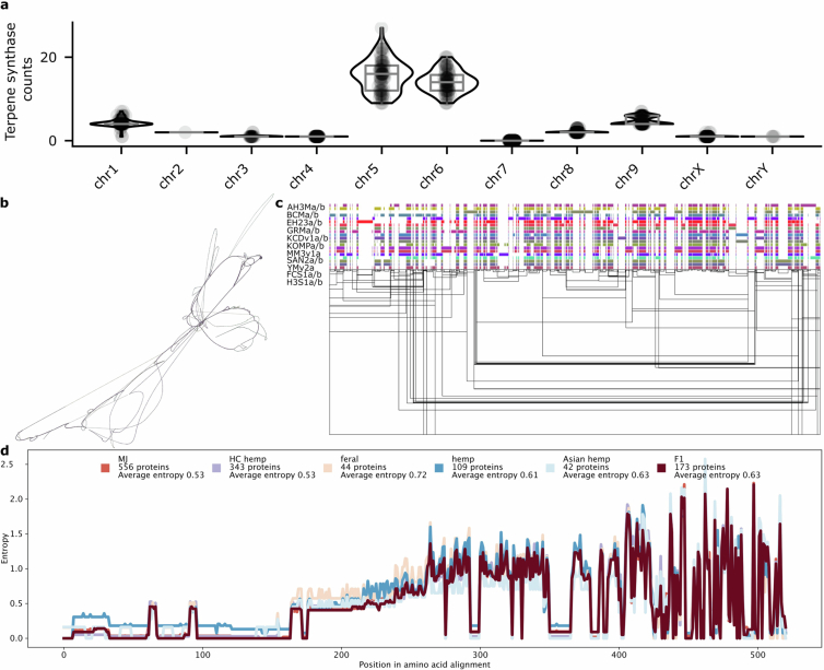
In planta cannabinoid alkyl side-chain length can vary from one to at least seven carbons, with five carbons being the most common in modern gene pools⁵². Three-carbon side-chain cannabinoids (propyl; tetrahydrocannabivarin (THCV), cannabivarin (CBDV) and cannabigerovarin (CBGV)) are much less common, but have attracted interest as novel therapeutic agents⁵³. Prior studies have characterized the polygenic nature of this trait, and associated the β-keto acyl carrier protein reductase (BKR) gene with varin cannabinoid production, but left open at least one step needed for a complete biosynthetic hypothesis⁵⁴. We extended the model for varin cannabinoid production by identifying a complex of acyl-lipid thioesterase (ALT3 and ALT4) genes located near the beginning of chr. 7 that were associated with varin production in our F₂ mapping population and were contained within a common haplotype in our k-mer-based crossover analysis of trios (Fig. 5, Supplementary Note 1, Supplementary Figs. 24–26 and Supplementary Tables 15 and 16). There was high ALT gene copy number variation in cannabis, ranging from 2–14 copies (considering both phased and unphased assemblies) across 4 chromosomes (Fig. 4a). Most plant genomes contain 4–5 ALT homologues, and some contain only a single homologue (for example, Brassica rapa and Glycine max)⁵⁵. Additionally, ALT protein sequence variation in cannabis was notable, with distinct orthogroup membership of each ALT4 in EH23a and EH23b genomes (Fig. 5b,c), despite these genes being located at similar positions (Fig. 5b). Since the shortest known fatty acid product of a plant fatty acyl-thioesterase is a 6:0 fatty acid generated by the Arabidopsis ALT4, the EH23a ALT4 allele is a lead candidate for further experimentation. However, given the crossover locations (Fig. 5a), potential for linkage disequilibrium and short-read mapping issues in this region, any of these ALT3 and ALT4 trans-duplicated genes (or splice variants) could be causal for varin cannabinoid production. Alternatively, they may have overlapping sub-functionalized substrate specificities, which would pose challenges for further mapping and improvement efforts⁵⁶.

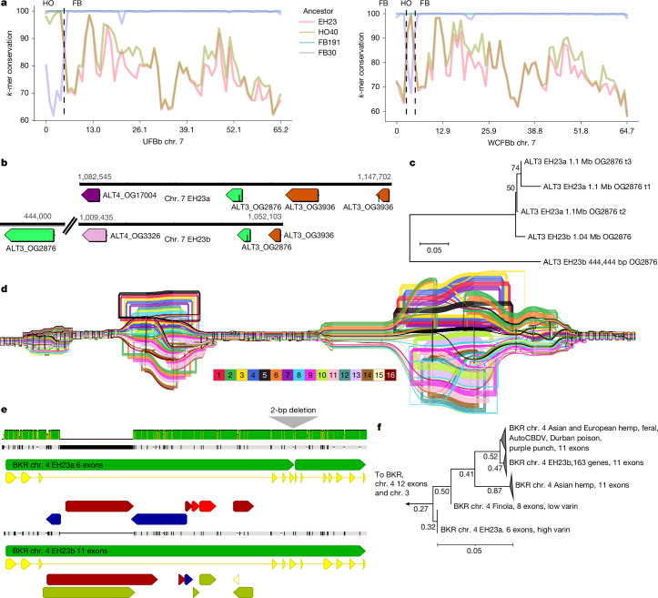
Although the BKR gene on chr. 4 was identified previously in a genome-wide association study, the pangenome showed that a 2-bp deletion produced a 6-exon loss-of-function gene model, which lacked catalytic active site residues (Fig. 5e). Thus, reduction or loss of function in this gene is probably required to increase the butyryl-acyl carrier protein pool, which one of the ALT3 or ALT4 gene products then hydrolyses to butyric acid, leading to varin cannabinoid biosynthesis (Fig. 4a). Since cannabis hosts BKR genes on chr. 3 and chr. 4, loss of catalytic function of one copy is unlikely to fully terminate iterative fatty acid chain synthesis, which could also explain why varin cannabinoids are only found in certain ratios with pentyl cannabinoids^52,54. Across the pangenome, the EH23a 6-exon BKR variant was exclusively found in HO40 pedigree samples (high varin); all other samples, except one 8-exon version of BKR in the seed oil cultivar Finola (low varin producer) were 11- or 12-exon models. The phylogenetic relationships of the predicted BKR proteins showed that the 6-exon gene may be closer to certain Asian hemp, European hemp and feral variants (Fig. 5f). However, one of the 11-exon gene clades contained the varin-producing AutoCBDV genome, and the potential varin producer Durban Poison, which could be reduced-function variants. Some reports suggest that there is no defined geographic origin associated with the varin chemical phenotype⁵⁷. However, other studies report plants that contain high levels of varin cannabinoids from the southern regions of Africa and certain regions of Asia^52,58. Collectively, the BKR gene phylogeny and whole-genome k-mer-based clustering analysis suggest an Asian origin for varin cannabinoid genes used in this breeding project (Fig. 1f,g). Deeper understanding of these biosynthetic pathways enhances our ability to select and optimize diverse cannabinoid production and suggests a path toward improvement of seed oil lipid profiles.

Conclusions

Our analysis of 193 cannabis genomes revealed that global diversity remains undersampled, with Asian germplasm notably underrepresented. Despite its phenotypic similarity to European hemp, Asian hemp carries highly divergent genomic regions, some of which align more closely with North American drug-type cannabis, suggesting undiscovered wild relatives and unresolved taxonomy. TE activity and hybridization, rather than whole-genome duplication, drive cannabis genome evolution. SVs uncover previously hidden diversity missed by short-read sequencing. Whereas cannabinoid synthase genes show limited variation, genes related to fatty acid metabolism, growth, defence and terpene biosynthesis exhibit extensive diversity and copy number variation. We assembled fully phased cannabis X and Y chromosomes, identifying a variable SDR–PAR boundary and unique male-specific homologues on the large Y chromosome that may influence flowering time and development, offering new targets for breeding.

Finally, the discovery of extensive variation in fatty acid biosynthesis genes (for example, ALT and BKR) suggested that cannabis has untapped potential for lipid metabolism. Given the overlap between cannabinoid biosynthesis and seed oil pathways, hybridizing diverse parental lines beyond the conventional Northern European hemp seed oil gene pool could yield novel lipid profiles and traits. The conservation and utilization of Asian hemp and wild cannabis will be critical for advancing cannabis breeding and the development of agronomic and pharmaceutical potential.

Methods

Plant material

C. sativa pangenome samples were selected from multiple sources to maximize the genetic diversity, history and agronomic value. A large portion of the pangenome comes from the Oregon CBD (OCBD) breeding programme that includes elite cultivars; foundational marijuana lines potentially originating from the 1970s to the present; and elite trios used for different aspects of the breeding programme (Extended Data Figs. 1 and 2, Supplementary Table 1 and Supplementary Fig. 1). The remaining cultivars come from the US Department of Agriculture (USDA) Germplasm Resource Information Network (GRIN) and German Federal Genebank (IPK Gatersleben) repositories, as well as collections made by the Salk Institute from various breeders. The pangenome includes European and Asian fibre and seed hemp, feral populations, North American marijuana (type I) and North American high cannabinoid yielding (CBD or CBG) hemp (type III and IV). Additional cannabinoid diversity is represented with chemotypes presenting high expression of pentyl or propyl (varin) homologues of CBD or THC, and cannabinoid-free (type V) plants. Flowering time variation is also captured with the inclusion of both regular short-day and day-neutral (autoflowering) phenotypes (Supplementary Table 1).

EH23 phased, haplotype-resolved, chromosome-scale anchor genome

EH23a (HO40) and EH23b (ERB) are haplotype-resolved assemblies for ERBxHO40_23, an F₁ resulting from a cross between parents, ERB and HO40, both proprietary female inbred lines from OCBD. ERB is a DN (autoflower), type III (CBDA-dominant) plant that is part of the drug-type group more closely related to European HC hemp. HO40 is type I propyl cannabinoid (THCVA and THCA)-producing, short-day flowering responsive, and is part of the drug-type marijuana group (MJ) with a closer affinity to Asian hemp. The genetically female (XX) ERB plant was induced to produce male flowers by treatment with silver thiosulfate and used to pollinate HO40. One individual from the F₁ populations (ERBxHO40_23) was selected for genome sequencing. Initial genome size estimates of ERB × HO40_23 using flow cytometry estimated a diploid genome size of 1445.6 Mb (722.8 Mb haploid genome size). High molecular weight (HMW) DNA was extracted from leaf tissue. Following DNA extraction and library preparation (see ‘HMW DNA isolation and genome sequencing’) HiFi reads were generated on the Pacific Bioscience (PacBio) Sequel II. Hifiasm v0.16.1⁵⁹ was then used in conjunction with Hi-C reads to produce initial assemblies. After assembly, Hi-C reads were aligned to the Hifiasm_HiC contigs using the Juicer v1.6.2 pipeline⁶⁰ followed by ordering and orientation utilizing version 180922 of the 3D-DNA pipeline⁶¹. The scaffolded assemblies were then manually corrected using Juicebox v1.11.08⁶².

EH23 F₂ population

In addition to the whole-genome sequencing data described above, ERBxHO40_23 was self-pollinated using silver thiosulfate induced masculinization of select flowers, to create an F₂ mapping population. From this F₂ population, individuals were scored for autoflower and varin content, and sequenced using Illumina 100 bp reads by NRGene (Nrgene Technologies). Illumina WGS genotyping runs were performed on 288 plants from this population, plus the ERBxHO40_23 parent. Trim_galore was used to trim sequences using: –2 colour 20, resulting in 271 individuals for analysis⁶³. On average samples had 8.5× coverage. Minimap was used to align each sample to EH23b.softmasked.fasta. Freebayes was used to call variants: -g 4500 -0 -n 4 –trim-complex-tail –min-alternate-count 3⁶⁴. Bcftools was used to filter on QUAL > 20 scores (99% chance variant exists)⁶⁵. Finally, Vcftools⁶⁶ tools was then used to further filter SNPs: –remove-indels –minGQ 20 –maf 0.25 –max-missing 1 –min-alleles 2 –max-alleles 2 –stdout –recode⁶⁶; only sites that were scored as heterozygous (0/1) in ERBxHO40_23 sample were retained, resulting in 93,251 SNPs.

EH23 F₂ cannabinoid HPLC methods

High-performance liquid chromatography (HPLC) was conducted according to the protocol thoroughly described previously⁶⁷ to determine relative propyl and pentyl cannabinoid content in all the plants used in this study, including F₂ progeny. In short, mature flower tissue was collected from each individual, frozen at −80 C and homogenized, before cannabinoids were extracted in methanol.

EH23 RNA sequencing

ERBxH040-21 seedlings were grown under controlled environmental conditions. Various tissues were collected during the development of the plants, including early and late flowers, foliage, foliage under a 12-h inductive light regimen, roots and shoot tips. Total RNA extraction was done using the QIAGEN RNeasy Plus Kit following manufacturer protocols. Total RNA was quantified using Qubit RNA Assay and TapeStation 4200. Prior to library prep, we performed DNase treatment followed by AMPure bead clean up and QIAGEN FastSelect HMR rRNA depletion. Library preparation was done with the NEBNext Ultra II RNA Library Prep Kit following manufacturer protocols. Then these libraries were run on the NovaSeq6000 platform in 2× 150-bp configuration.

EH23 haplotype expression analysis

We measured gene expression levels using Salmon v1.6.0⁶⁸. In brief, the raw paired end short reads from sequencing were mapped to the CDSs from both haplotypes (EH23a and EH23b) and the abundance was estimated in transcripts per million (TPM) for downstream analysis. Mapping rates were calculated with samtools flagstat⁶⁵. The minimum TPM threshold for a given gene was ≥0.1. Haplotype gene pairs were identified by reciprocal best hits and synteny using blastp and MCScanX⁶⁹, and only genes shared between both haplotypes were included. A minimum of ≥95% sequence similarity and a threshold of 5 TPM difference between haplotypes was imposed. Visualization was performed using a combination of Matplotlib⁷⁰, SciPy⁷¹ and NumPy⁷², and expression values are shown in heat maps as log₂TPM to represent log fold change. Enrichment of Biological Processes GO Terms was performed with topGO⁷³ with the following parameters: resultWeight <- runTest(topGOdata, algorithm = “weight01”, statistic = “fisher”). A multiple test correction was performed with the following command: fullResults$p.adj <- p.adjust(as.numeric(fullResults$weightFisher), method = “fdr”). The background gene universe included all genes with a GO term from either EH23a or EH23b.

Ace High sex-biased gene expression analysis

We collected flower and leaf tissue from four Ace High plants, two male and two female, at the same developmental time point, at 08:00 and 20:00, for a total of 16 samples. Since Ace High males flower several weeks before female plants under normal outdoor conditions, plants were germinated and grown under long days and transferred to inductive short-day conditions for flowering, which resulted in both male and female plants developing flowers at the same time. Samples were collected at two times of day to capture all transcripts regardless of their circadian or diurnal expression⁷⁴. RNA was extracted with the Qiagen Plant RNA kit. Library prep was performed with the Oxford Nanopore Technologies (ONT) full-length cDNA kit. We aligned full-length cDNA to the haplotype-resolved Ace High (AH3Ma/b) genomes with minimap2 (v2.24)⁷⁵ and gene expression was measured using Salmon v1.6.0⁶⁸. Sex-biased expression was assigned for all tissue-specific male and female samples (leaf and flower from two male plants (plants A and B, collected at 08:00 and 20:00) and two female plants (plants C and D, collected at 08:00 and 20:00)). Each sex-specific tissue had four replicates (for example, gene expression measurements from male flowers sampled from two male plants at two different time points were averaged). Two categories of biased expression were defined: first, average expression that was higher (at least 5.0 TPM greater) in male or female samples, relative to the other sex; and second, male or female-only expression, where genes were not expressed in one sex (0.0 TPM for all replicates), but had an average of at least 1.0 TPM expression in the other sex. For GO term analysis with topGO⁷³, both categories of biased gene expression were combined. Fully syntenic genes were identified in the set of four genomes with X and Y chromosomes (AH3Ma/b, BCMa/b, GRMa/b and KOMPa/b) using genespace, and were grouped according to location in the PAR, SDR or X-specific region.

Hi-C library preparation and sequencing

For the Dovetail Omni-C library, chromatin was fixed in place with formaldehyde in the nucleus and then extracted. Fixed chromatin was digested with DNAse I, chromatin ends were repaired and ligated to a biotinylated bridge adapter followed by proximity ligation of adapter containing ends. After proximity ligation, crosslinks were reversed and the DNA purified. Purified DNA was treated to remove biotin that was not internal to ligated fragments. Sequencing libraries were generated using NEBNext Ultra enzymes and Illumina-compatible adapters. Biotin-containing fragments were isolated using streptavidin beads before PCR enrichment of each library. The library was sequenced on an Illumina HiSeqX platform to produce ~30× sequence coverage. Then HiRise used (see read-pair above) MQ > 50 reads for scaffolding. Additional Hi-C libraries were generated using Phase Genomics Proximo Hi-C Kit (Plant) version 4.

HMW DNA isolation and genome sequencing

All samples were sequenced on a PacBio Sequel II. For samples sourced from ‘Michael’ (Supplementary Table 1), HMW DNA was isolated using Carlson Lysis buffer and Qiagen Genomic tips as described in the ONT Protocol ‘Plant leaf gDNA’ Arabidopsis method. The DNA was further size-selected for fragments longer than 10–25 kb using the ONT Short Fragment Eliminator Kit (EXP-SFE001). HMW DNA was then confirmed by Tapestation Genomic DNA ScreenTape (Agilent 5067-5365) or Femto Pulse Genomic DNA 165 kb Kit (Agilent FP-1002-0275). For samples sourced from ‘OCBD’ (Supplementary Table 1), HMW DNA was isolated using a modified protocol⁷⁶. In brief, samples were ground in a mortar and pestle with liquid nitrogen, two chloroform:isoamyl wash cycles were performed, and Total Pure NGS beads (Omega Biotek) were used as a substitute from the original protocol. Genomic DNA (gDNA) quality and purity was then assessed using a NanoDrop One (ThermoFisher) prior to starting library preparation. Continuous long read (CLR) libraries were made using the Pacbio protocol PN 101-693-800 V1. Size selections on gDNA were made using the Blue Pippin U1 High Pass 30–40 kb cassette with a 30–40 kb base pair starting threshold to produce fragment distributions of 60–90 kb. HiFi circular consensus sequencing (CCS) libraries were prepared according to the PacBio protocol (PN 101-853-100 V5). Sheared gDNA fragment distributions with a modal peak ~18 kb were produced using g-Tubes from Covaris and Blue Pippin S1 High Pass 6–10 kb cassettes to remove everything under 10 kb in size.

Pangenome assembly and scaffolding

All genomes labelled Hifiasm_HiC, Hifiasm_Trio_RagTag, Hifiasm_RagTag, and Hifiasm (Supplementary Table 1) were assembled using Hifiasm v0.16.1⁵⁹. When available, Hi-C data and HiFi parental trio data were also incorporated into the assembly process defining the Hifiasm_HiC and Hifiasm_Trio_RagTag types respectively. CLR assemblies were generated using FALCON Unzip from PacBio SMRT Tools 9.0 Suite⁷⁷ and CCS labelled genomes were assembled with HiCanu v2.2⁷⁸. After assembly, Hi-C reads were aligned to the Hifiasm_HiC contigs using the Juicer v1.6.2 pipeline⁶⁰ followed by ordering and orientation utilizing version 180922 of the 3D-DNA pipeline⁶¹. The scaffolded assemblies were then manually corrected using Juicebox v1.11.08⁶². Hifiasm_RagTag and Hifiasm_Trio_RagTag assemblies were scaffolded using the split chromosomes of the 24 Hi-C scaffolded genomes and error checked with yak-0.1 (github.com/lh3/yak). Sourmash v4.6.1⁷⁹ was used to generate a Jaccard similarity matrix between the chromosomes and each un-scaffolded assembly, and the most similar version of chromosome 1 through X was concatenated to generate a reference for scaffolding via RagTag v2.1.0⁸⁰. If the similarity matrix identified the Y chromosome as the best match, the assembly remained un-scaffolded. BUSCO v5.4.3⁷⁹ with the eudicots_odb10 dataset and assembly-stats v1.0.1 (https://github.com/sanger-pathogens/assembly-stats) were used on all assemblies to measure completeness and contiguity.

Reference-based graph construction with Minigraph-cactus

The graph pangenome of all 78 scaffolded and softmasked assemblies was generated with Minigraph-Cactus²⁰. We used the cactus-pangenome command within an Apptainer (v1.1.8) Image⁸¹ (https://quay.io/comparative-genomics-toolkit/cactus:v2.6.7-gpu) and the following parameter flags: –reference EH23a EH23b –vcf –vcfReference EH23a EH23b –giraffe –chrom-og –chrom-vg –viz –gfa –gbz. The seqFile input as well as the output graph in various formats (vg, paf, hal, etc.) can be found at https://resources.michael.salk.edu. We also compiled variants across the pangenome in terms of each assembly’s coordinates by using vg deconstruct -a -C (vg tools v1.61.0 “Plodio”) to derive vcf files from the Minigraph-Cactus gfa output and then using vcfbub –max-ref-length 100000 –max-level 0 to flatten nested variants and remove those >100 kb in length (see 78csatHaps_minigraphcactus_<assembly>.vcf.gz)^20,82,83.

Reference-free graph construction with PGGB

Input sequences and orientation

We generated two versions of each PGGB graph, one with the fasta files provided in the ‘Assembly files’ table and in the JBrowse instance at https://resources.michael.salk.edu (mixed-orientation) and one with fasta files in which the sequences have been consistently oriented to match the plus strand of the corresponding homologous chromosome in EH23a (consistent-orientation).

For PGGB graph 16csatAsms, we generated one graph per autosomal chromosome from the following 16 scaffolded and softmasked assemblies: AH3Ma, AH3Mb, BCMa, BCMb, EH23a, EH23b, GRMa, GRMb, KCDv1a, KCDv1b, KOMPa, KOMPb, MM3v1a, SAN2a, SAN2b and YMv2a. We generated one combined fasta file per chromosome as inputs for PGGB (see 16csatAsms_chr[1-9]_combined.fa.gz and 16csatAsms_chr[1-9]-oOrient_combined.fa.gz for the consistent- and mixed-orientation fasta inputs, respectively, at resources.michael.salk.edu). We constructed per chromosome graphs instead of a single graph for the entirety of all assemblies combined due to the computational requirements for analysing genomes of this size and repetitive content (Extended Data Fig. 6).

For PGGB graph 13csatSexChroms, the 13 scaffolded and softmasked sex chromosome sequences AH3Ma.chrX, AH3Mb.chrY, BCMa.chrX, BCMb.chrY, EH23a.chrX, GRMa.chrY, GRMb.chrX, KCDv1a.chrX, KCDv1b.chrX, KOMPa.chrX, KOMPb.chrY, SAN2a.chrX and SAN2b.chrX were combined into one fasta file (see 13csatSexChromsCombined_filtOrientation.fa.gz and 13csatSexChromsCombined_origOrientation.fa.gz for the consistent- and mixed-orientation fasta inputs, respectively, at https://resources.michael.salk.edu).

Graph generation

Nextflow v24.04.3.5916⁸⁴ was used to run the nf-core/pangenome v1.1.2 – canguro deployment^85,86 of PGGB²² within the nextflow singularity profile. All default PGGB settings were used for graph generation. For PGGB graph 13csatSexChroms, the flag –vcf_spec was used to compile sequence variation across the pangenome relative to each assembly’s coordinates, and each vcf was further processed with vcfbub –max-ref-length 100000 –max-level 0 to flatten nested variants and remove those >100 kb in length²⁰ (see 13csatSexChroms_pggb-fOrient_<assembly>.vcfbub.vcf.gz and 13csatSexChroms_pggb-oOrient_<assembly>.vcfbub.vcf.gz files for vcfs from graphs generated with consistent- and mixed-orientation input fastas, respectively, at https://resources.michael.salk.edu). For PGGB graph 16csatAsms, PGGB was run without the flag –vcf_spec and, instead, vg deconstruct -a was used to compile sequence variation across the pangenome from the final gfa file for each autosomal chromosome (vg tools v1.61.0 “Plodio”)^82,83. Per-autosome vcf files were concatenated into a single file for each assembly using bcftools⁶⁵ and then processed with vcfbub –max-ref-length 100000 –max-level 0 to flatten nested variants and remove those >100 kb in length²⁰ (see 16csatAsms_pggbByChrom_<assembly>.vcf.gz and 16csatAsms_pggbByOriginalChrom_<assembly>.vcf.gz for vcfs from graphs generated with consistent- and mixed-orientation input fastas, respectively, at resources.michael.salk.edu). Identical parameters were used for each pair of graphs generated with consistent- and mixed-orientation inputs.

Visualization

Visualizations of the graph pangenomes were generated from the FINAL_GFA files of the PGGB pipeline run on consistent-orientation input fastas. Vg files were derived from gfa files using vg convert^82,83. Then prepare_vg.sh and prepare_chunks.sh were used to visualize the pangenome variation at regions of interest in a local instance of the Sequence Tube Map server (https://github.com/vgteam/sequenceTubeMap.git, cloned on 4 September 2024).

Short-read mapping to graph pangenome

Short-read sequences from the EH23 F₂ population and Ren et al.² were aligned to the pangenome graph with vg giraffe (example command: vg giraffe -Z {input.inputGBZ} -d {input.inputDist} -m {input.inputMin} -f {input.inputR1} -f {input.inputR2} -t {threads} > {output.outputFile})⁸⁷. Summary statistics were collected with vg stats⁸² (example command: vg stats -a {input.inputGAM} {input.inputGBZ} > {output.outputFile}). Calculate read support from GAM file with vg pack⁸² (example command: vg pack -x {input.inputGBZ} -g {input.inputGAM} -Q 5 -t {threads} -o {output.outputFile}). Variants for the F₂ mapping population were called with vg call⁸⁸ (example command: vg call –gbz {input.inputGBZ} -k {input.inputPack} -S EH23b -t {threads} > {output.outputFile}). Downstream processing of VCF files was performed with BCFtools⁶⁵ (example commands: (1) bcftools view -a -f PASS merged.sorted.vcf.gz > merged.sorted.a.PASS.vcf.gz; (2) bcftools norm –fasta-ref EH23b.softmasked.fasta -m -any merged.sorted.a.PASS.vcf.gz > merged.sorted.a.PASS.normed.vcf.gz; (3) bcftools norm –fasta-ref EH23b.softmasked.fasta –rm-dup exact merged.sorted.a.PASS.normed.vcf.gz > merged.sorted.a.PASS.normed_no_dups.vcf.gz). Filtering of the pangenome graph-based VCF file to compare with the linear reference-based VCF file was performed with VCFtools⁶⁶ (example command: vcftools –remove-indels –minGQ 20 –maf 0.25 –max-missing 0.3 –min-alleles 2 –max-alleles 2 –stdout –recode –gzvcf merged.sorted.a.PASS.normed_no_dups.vcf.gz > merged.sorted.a.PASS.normed_no_dups.more_filter_missing0.3.vcf.gz).

Graph pangenome data availability

Input and output files for the graph pangenomes described above (78csatHaps generated by Minigraph-Cactus, and 16csatAsms and 13csatSexChroms generated by PGGB) are available at https://resources.michael.salk.edu. Vcf files have been added as tracks to the Cannabis genomes JBrowse instance at https://resources.michael.salk.edu.

Base-calling methylated cytosines

Genomic reads from the raw ONT FAST5 files generated from Cannabis sequencing samples were used for methylation calling. Genome assemblies generated for the same individuals were used as references for alignment. FAST5 data were converted to POD5 format using the pod5 software package (https://github.com/nanoporetech/pod5-file-format). Methylation calling was performed with ONT base-calling software Dorado version 0.3.4 (https://github.com/nanoporetech/dorado/). Dorado uses the raw POD5 data and a reference to identify methylated cytosines. This was performed with the super high accuracy (SUP) base-calling model trained for R9.4.1 or R10.4.1 pore type and 400 bps translocation speed, according to the sequencing conditions for each line. The assembled genomes generated from each sample were used as references to generate an aligned BAM file with MM/ML tags containing 5mC and 5hmC methylation calls. These were then piled up with modkit (https://github.com/nanoporetech/modkit), and the piled-up calls (aggregating 5mC with 5hmC) were used for calculating genome-wide methylation frequencies across all CG sites.

Gene and repeat prediction

Gene model prediction involved a multi-step pipeline and was applied to all assemblies.

1. We first curated a repeat library using RepeatModeler⁸⁹ on a small number of high-quality Cannabis assemblies and pre-existing repeat libraries. We used OrthoFinder (v2.5.4)⁹⁰ to group repeats for deduplication. The final repeat library included 10% of the sequences from each repeat orthogroup (minimum 1 sequence) for a total of 6,262 sequences from 5,793 groups.
2. For all 193 genomes, repeats were masked with RepeatMasker (v4.1.2)⁹¹ using the repeat library (above).
3. We predicted gene models with the TSEBRA pipeline (using Braker v2.1.6)⁹². We developed a Snakemake workflow for running TSEBRA, available here: https://gitlab.com/salk-tm/snake_tsebra. We incorporated a variety of pre-existing protein libraries from cannabis and other organisms as evidence: (a) Arabidopsis thaliana; (b) Theobroma cacao; (c) G. max; (d) Rhamnella rubrinervis; (e) Ziziphus jujuba; (f) Trema orientale; (g) Vitis vinifera; (h) Prunus persica; (i) Morus notabilis; (j) C. sativa; (k) H. lupulus.
4. RNA-seq libraries (Supplementary Table 2) were aligned with either hisat2 (v2.2.1)⁹³ for short-read mapping, or minimap2 (v2.24)⁷⁵ for full-length cDNA. Short-read Illumina data was trimmed with fastp⁹⁴. The expression data was incorporated into the TSEBRA pipeline as gene model evidence.
5. Putative functional annotations of gene models were assigned using eggnog-mapper (v2.0.1)⁹⁵.
6. Overall gene model quality and completeness was assessed by comparing genome BUSCO (v5.4.3)⁹⁶ scores to proteome BUSCO scores on the eudicots_ocdb10 dataset (Supplementary Table 1: 10.6084/m9.figshare.25869319.v2).
7. EDTA v1.9.6⁹⁷ was also utilized to identify TEs in the cannabis pangenome with the following command: EDTA.pl –genome {inputFastaFile} –anno 1 –threads 32.

Ideogram methods

Ideograms for each pair of chromosomes for the 78 chromosome-level, haplotype-phased genomes were created using ggplot2 [https://ggplot2.tidyverse.org] in R (www.R-project.org) (Fig. 1 and Extended Data Fig. 5). The length of each chromosome was determined using ‘nuccomp.py’ (https://github.com/knausb/nuccomp) and used with ggplot::geom_rect() to initialize the plot. One million base pair windows were created for each chromosome where the number of CpG motifs were counted for each window with the program motif_counter.py (https://github.com/knausb/nuccomp). The CpG count was converted into a rate by dividing by the window size; this also accommodated the last window of each chromosome, which was less than one million base pairs in size. These rates were scaled by subtracting the minimum rate and then dividing by the maximum rate (the maximum rate after subtracting the minimum rate), on a per chromosome basis. In order to visually emphasize the enrichment of the CpG motif in the centromeric region, an inverse of the CpG rate was taken by taking one and subtracting the CpG rate for each window. This scaled, inverse CpG rate was used for the width of each one mbp window and coloured based on gene density using the viridis magma palette (10.5281/zenodo.4679424).

Structural variation among each pair of chromosomes was determined using minimap2⁷⁵ alignments. The minimap2 comparisons were annotated using SyRI⁹⁸. The syntenous and inverted regions were plotted using ggplot2::geom_polygon() in a manner inspired by plotsr⁹⁹ but implemented in R (github.com/ViningLab/CannabisPangenome).

The location of candidate loci within EH23 haplotypes A and B were determined using BLASTN¹⁰⁰. Query sequences were as follows: CBCA synthase (LY658671.1), CBDA synthase (AB292682, AB292683, AB292684), THCA synthase (AB212829, AB212830), and olivetolic acid cyclase (NC_044376.1:c4279947-4279296, NC_044376.1:c4272107-4271242). These sequences were combined with centromeric, telomeric and rRNA sequences in the file blastn_queries_rrna_cann.fasta (https://github.com/ViningLab/CannabisPangenome). BLASTN was called with the following options: -task megablast -evalue 0.001 -perc_identity 90 -qcov_hsp_perc 90. Tabular results (subject chromosome, subject start of alignment, subject end of alignment) from BLASTN were read into R and plotted on ideograms with ggplot2::geom_rect() (https://ggplot2.tidyverse.org).

Centromere and telomere analysis

ONT and PacBio based long read-based genome assemblies enable the assembly of some of the highly repetitive centromeres and telomeres sequences¹⁰¹. Centromeres were identified by searching genomes using tandem repeat finder (TRF; v4.09) using modified settings (1 1 2 80 5 200 2000 -d -h)¹⁰². Tandem repeats were reformatted, summed and plotted to find the highest copy number tandem repeat per our previous methods to identify centromeres¹⁰¹ (Extended Data Fig. 5c).

Telomeres were estimated using two different methods. First, the TRF output was queried for repeats with the period of 7 for the 14 different version of the canonical telomere base repeat: AAACCCT, AACCCTA, ACCCTAA, CCCTAAA, CCTAAAC, CTAAACC, TAAACCC, TTTAGGG, TTAGGGT, TAGGGTT, AGGGTTT, GGGTTTA, GGTTTAG and GTTTAGG: (grep -a ‘PeriodSize=7’ *.genome.fasta.1.1.2.80.5.200.2000.dat.gff | grep -a ‘Consensus=AAACCCT\|Consensus=AACCCTA\|Consensus=ACCCTAA\|Consensus=CCCTAAA\|Consensus=CCTAAAC\|Consensus=CTAAACC\|Consensus=TAAACCC\|Consensus=TTTAGGG\|Consensus=TTAGGGT\|Consensus=TAGGGTT\|Consensus=AGGGTTT\|Consensus=GGGTTTA\|Consensus=GGTTTAG\|Consensus=GTTTAGG’ -). Second, we searched raw ONT and PacBio reads for telomere sequences using our TeloNum algorithm¹⁰³. Although the results were variable across the pangenome assemblies, in general, telomere sequence was found at the end of the chromosome with an average length of 16 kb for PacBio assemblies and 60 kb for ONT assemblies. The differences between ONT and PacBio telomere length most likely reflected the input read length of >100 kb and 15–20 kb, respectively. TeloNum analysis of the raw reads supported the distributions from the assemblies consistent with most chromosomes having telomere sequence while being shorter than the actual size. Cannabis telomeres are on the longer side for a eudicot and could be explained by its predominantly clonal propagation for medicinal uses¹⁰⁴.

Centromere sequence was identified based on the hypothesis that it will be the most abundant repeat in the genomes that also has a higher-order repeat (HOR) structure^101,105. Two different repeats with HOR were identified in the PacBio HiFiasm assemblies, whereas only one was found in the ONT assemblies and the previous CBDRx assembly, which is based on ONT sequence¹¹. The highest copy number repeat was 370 bp that varied between 20–30 Mb (2–4% of the total genome) with HOR at 740 and 1,110 bp (Extended Data Fig. 5). The second highest, and the only one found in the ONT assemblies, was a 237 bp repeat that varied between 3–5 Mb (0.4–1.0% of the total genome) and had HOR at 474 and 711 bp (Extended Data Fig. 5). Mapping of the 370-bp repeat to the chromosome-resolved genomes revealed that this repeat was primarily located at the end of the chromosomes next to the telomere sequence, which suggested that it may be related to the CS-1 sub-telomeric repeat¹⁰⁶. Comparison of the putative 370-bp centromeric repeat and the CS-1 sub-telomeric repeat showed they are the same repeat element. By contrast, the putative 237-bp centromeric repeat predominantly was found on chr. 6 and chr. 8 in the predicted centromere region (Fig. 1a and Extended Data Fig. 5). However, smaller 237-bp arrays were found on all chromosomes across the assemblies in the predicted centromere region (based on CpG, methylation, gene content and TEs) with most assemblies having small arrays on chr. 6 and chr. 8.

Ribosomal DNA detection and quantification

Ribosomal DNA (rDNA) 45S (18S, 5.8S and 26S) and 5S sequences were identified in the CBDRx/CS10 assembly (LOC115701787 5.8S, LOC115701759 18S, LOC115701762 26S and LOC115721558 5S) and used to BLAST against the pangenome assemblies (Fig. 1a and Extended Data Fig. 5). Across the scaffolded genomes the 45S array was predominantly located on the acrocentric end of chr. 8, and the 5S was located exclusively on chr. 7 between the cannabinoid synthase cassette array, consistent with published results with fluorescence in situ hybridization¹⁰⁶. However, partial arrays were found in some assemblies on all of the chromosomes (Extended Data Fig. 5). The distribution of the partial arrays on different chromosomes could reflect variability across the genomes since some share similar locations across assemblies. Most arrays are found on the un-scaffolded contigs, suggesting that these variable arrays across different chromosomes could be the result of mis-assemblies. In general, there are on average 1,000 45S and 2,000 5S arrays in the cannabis genome; some assemblies have the 5S array completely assembled on chr. 7.

Allele frequency methods

Genotype data in the VCF format¹⁰⁷ was input into R using vcfR¹⁰⁸. Allele and heterozygous counts were made with vcfR. Wright’s F_IS was calculated¹⁰⁹ to provide the deviation in heterozygosity from our random, Hardy–Weinberg, expectation. Wright’s F_IS was calculated as (HS − HO)/HS, where HO is the observed number of heterozygotes divided by their number and HS is the number of heterozygotes we expect based on the allele frequencies, calculated as the frequency of the first allele multiplied by the frequency of the second multiplied by two and divided by their number. Scatter plots were generated using ggplot2. Graphical panels were assembled into a single graphic using ggpubr (https://cran.r-project.org/package=ggpubr).

PanKmer genome analysis

Using PanKmer, we constructed two 31-mer indexes: a ‘full’ index of 193 Cannabis assemblies and a ‘scaffolded-only’ index of 78 scaffolded assemblies, using the ‘pankmer index’ command with default parameters. We calculated and plotted pairwise Jaccard similarities for all assemblies in the full index using ‘pankmer adj-matrix’ followed by ‘pankmer clustermap –metric jaccard’. We calculated and plotted a collector’s curves for both the full and scaffolded-only indexes using the ‘pankmer collect’ command with default parameters. All scripts used for this analysis can be found on GitHub.

Analysis of gene-based pangenome

We define the gene-based pangenome as the set of all gene families (orthogroups) with a representative in at least one genome of the pangenome. For each of 193 (as well as the 78 chromosome-level, haplotype-phased genomes, as a separate set) C. sativa genomes, the primary transcript of each high-confidence gene prediction was chosen as a representative. The proteins corresponding to each primary transcript were clustered into orthogroups using Orthofinder (v.2.5.4, see Orthofinder and synteny analysis section below)⁹⁰. The set of primary transcript CDS were merged into a single FASTA file, and exact duplicates were removed with SeqKit (2.7.0)¹¹⁰. Among primary transcripts, likely contaminants were determined by identifying transcripts predicted on contigs where fewer than 90% of predictions were annotated as either ‘viridiplantae’ or ‘eukaryote’ according to eggNOG-mapper (v2.1.12)⁹⁵, and were removed. To mitigate the problem of unannotated genes, we aligned coding sequences of all primary transcripts to each of the 193 (78) cannabis genomes using minimap2 (v2.26)⁷⁵ with parameters ‘minimap2 -c -x splice’ to generate a PAF file with CIGAR strings for each genome. For each genome, if an aligned CDS sequence had a mapping quality of at least 60, had a number of CIGAR matches at least 80% of the query length, and did not overlap a directly annotated gene, it was considered an unannotated gene and its orthogroup was marked as present in the target genome. The set of orthogroups that had at least one representative present in all 193 (78) genomes were considered to be the core genome, the remaining orthogroups were considered to be the variable genome. The presence or absence of each orthogroup in each genome was recorded in a table (see Data availability). All scripts for this analysis are available from GitHub.

Haplotypes, orthogroups and scores

In pangenomics, collector’s curves (pangenome rarefication) show the relationship of the number of haplotypes (here H) to the number of gene families or orthogroups (here X).

Given the X orthogroups distributed across H haplotypes, let the score s_x ∈ [0, H] of an orthogroup x be the number of haplotypes in which x is present. For any score s let P(s) be the number of orthogroups with score equal to s.

Where I_{s_x}:{x₀…x_X} → {0,1} is the indicator function on {x ∈ x₀…x_X: s_x = s}.

The collector’s curves

The collector’s curve C(h): [1, H] → [0, X] is the expected number of orthogroups that will be present in a subset of h haplotypes randomly drawn from the total set of H. It can be calculated by:

The expected number of core orthogroups \({C}^{\wedge }(h)\) can be estimated by

Each of these is a special case of a general formula for the expected number of orthogroups with a score of at least n, based on the hypergeometric survival function:

Where S_hyp is the hypergeometric survival function or the hypergeometric cumulative distribution function subtracted from 1:

Where for clarity, the hypergeometric probability mass function (PMF) is:

With binomial coefficients defined as:

And, conventionally, the cumulative distribution function (CDF_hyp) is:

So defined, we can see that the pan-genome collector’s curve C(h) is equivalent to C₁(h), while the core genome collector’s curve \({C}^{\wedge }(h)\) is equivalent to C_h(h):

k-mer based collector’s curves

The definition of the collector’s curve is agnostic to the unit of genomic sequence, so the calculation of a k-mer based curve is identical to the orthogroup based curve, excepting that X will be the number of k-mers and x will represent a k-mer, rather than an orthogroup.

k-mer analysis of pangenome assemblies and global diversity short-read libraries

Trim_galore was used to trim Illumina short-read sequences from Ren et al.² using: –2 colour 20⁶³. These reads were next filtered for low abundance reads (trim-low-abund.py -C 10 -M 5e9), and then used to make a k-mer sketch (sourmash sketch dna -p scaled=1000,k = 31)⁷⁹. All pangenome assemblies were also analysed for 31-mer frequencies (sourmash sketch dna -p scaled=1000,k = 31). Finally, all pairwise samples of Illumina read and pangenome assemblies were compared (sourmash compare -p 64 *.sig -k 31). The 31-mer distances were then plotted in R using (hclust(dist(sourmash_comp_matrix), method = “average”)).

Identification of pangenome core and dispensable genes

We assigned core and dispensable (nearly-core, cloud, shell, private) genes based on orthogroup membership (https://github.com/padgittl/CannabisPangenomeAnalyses/tree/main/CoreDispensableGenes). Core genes were defined as being present in 100% of genomes (193 genomes), nearly-core genes were defined as being present in 95–99% of genomes (183–192 genomes), shell genes were found in 5–94% of genomes (10–182 genomes), cloud genes were found in 2–5% of genomes (3–9 genomes), and unique genes were found in 0.5–1% of genomes (1–2 genomes)¹¹¹. This analysis was performed on all 193 genomes (Fig. 1e) and also visualized according to population (Supplementary Fig. 5). For the contig-level assemblies (103 genomes), only contigs with similarity to the ten chromosomes of EH23a were included. Gene sets were filtered to include only genes that were present on the ten chromosomes and contigs homologous to the chromosomes. We performed an analysis of functional enrichment with topGO⁷³ for each of the core, shell, cloud, nearly-core, and unique gene groupings for each genome, where the background gene set was all genes with a GO term for a given genome. Among the core genes, the most common significant GO term in the pangenome was sesquiterpene biosynthetic process (GO:0051762), which was significant in all but one genome (PBBK), followed by GO:0045338 farnesyl diphosphate metabolic process, which was absent in three genomes (public genomes: CANN, FIN and PBBK) (Supplementary Table 4). This analysis was restricted to high-confidence gene models predicted with the TSEBRA pipeline. By contrast, the collector’s curve analysis of gene content also included unannotated genome regions lacking gene model predictions, but with similarity to known genes, as a way to capture unsampled diversity (Fig. 1c,d and Supplementary Fig. 4; see also ‘Analysis of gene-based pangenome’).

Repeat analysis

Calculation of divergence time in TEs

Estimates of divergence time shown (Fig. 2b,c) were calculated using the equation T = (1 − identity)/2µ, where identity was obtained from EDTA output GFF3 files described previously⁹⁷. We used a substitution rate (µ) of 6.1 × 10⁻⁹ from Arabidopsis^112,113. This analysis was performed on all genomes.

Identification of solo to intact LTR-RT ratio

To identify solo LTRs and intact LTR-RTs, we used the EDTA pipeline on 193 cannabis genomes⁹⁷. We identified solo LTRs by first collecting the set of LTRs that were not assigned as intact LTR-RTs, which are retrieved on the basis of ‘method=homology’ in the attribute column of the TEanno.gff3 file. We applied thresholds to isolate solo LTRs from truncated and intact LTRs, as well as internal sequences of LTR-RTs. These thresholds include a minimum sequence length of 100 bp, 0.8 identity relative to the reference LTR, and a minimum alignment score¹¹⁴ of 300. We also required that the four adjacent LTR-RT annotations did not have the same LTR-RT ID¹¹⁵. Further, we required a minimum distance of 5,000 bp to the nearest adjacent solo-LTR, intact LTR or internal sequence¹¹⁶. Last, we kept solo-LTR sequences that fell within the 95th percentile for LTR lengths¹¹⁷. Overall, this method represents a modified approach based on the solo_finder.pl script from LTR_retriever¹¹⁴ and the LTR_MINER script¹¹⁶ with guidance from the github page for LTR_retriever (https://github.com/oushujun/LTR_retriever/issues/41).

Enrichment of TEs flanking genomic features

The method presented as part of PlanTEnrichment¹¹⁸ was adapted for the cannabis pangenome to assess TE enrichment both upstream and downstream of different genomic features, including cannabinoid synthase genes. The goal of the analysis was to identify TEs that are significantly associated with a specific category of genomic feature. In brief, ‘X’ represents a specific type of TE and ‘Y’ encompasses all TEs. The total number of X located upstream or downstream of a specific genomic feature (for example, cannabinoid synthases) is denoted as a; the total number of X located upstream or downstream of all genomic features (for example, all genes) is b; the total number of Y located upstream or downstream of a specific genomic feature (cannabinoid synthases) is c; and the total number of Y located upstream or downstream of all genomic features (all genes) is d. An enrichment score (ES) is defined as \({\rm{ES}}=(a/b)/(c/d)\), and the P value is defined as \(p=(a+b)!(c+d)!(a+c)!(b+d)!/(a!b!c!d!N!)\), where N is the sum of a, b, c and d. A multiple test correction¹¹⁹ was performed on the P values using the Python library statsmodels¹²⁰. Significance threshold cut-offs included a false discovery rate (FDR) < 0.05 and ES ≥ 2. We used bedtools intersect¹²¹ to collect and survey the set of TEs located 1 kb upstream or downstream of the genomic feature category of interest. An example command: bedtools intersect -a assemblyID_genomic_feature_coord_file.txt -b assemblyID.TE.gff3 -wo > assemblyID_intersect_results.txt.

Distance between genes and TEs

The median and mean distances between genes and each of the TE categories was calculated using bedtools sort (bedtools sort -i genome.TEs.bed > genome.sorted.TEs.bed) and bedops closest-features (command: closest-features –closest –header –dist genome.sorted.genes.bed genome.sorted.TEs.bed > genome.closest_features.bed)¹²². To obtain the initial pre-sorted BED file for genes, the following command was used: cat genes.gff3 | grep mRNA | grep ‘\.chr’ | awk ‘{print $1”\t”$4”\t”$5”\t”$7”\t”$3”\t”$9}’ > genome.genes.bed. For TEs, the following command was used: cat genome.EDTA.TEanno.gff3 | grep ‘\.chr’ | awk ‘{print $1”\t”$4”\t”$5”\t”$7”\t”$3”\t”$9}’ > genome.TEs.bed. To calculate mean and median values, the built-in Python statistics module was used.

Enrichment of genes associated with different categories of TEs

We performed a GO term enrichment analysis to identify genes that were statistically significantly located near different types of TEs on the full pangenome. To identify genes near TEs, we first created a concatenated, sorted bed file with both gene and TE coordinates to find the nearest TE for a given gene, while excluding cases where the closest genomic feature to a given gene was another gene. For scaffolded genomes, genes and TEs were restricted to the ten chromosomes. For contig-level assemblies, genes were included if they were on a contig with similarity to one of the ten EH23a chromosomes. Next, we identified gene/TE pairs using bedops closest-features¹²². We performed a GO enrichment test for each genome separately using topGO with parameters algorithm = ‘weight01’, statistic = ‘fisher’, and Benjamini–Hochberg multiple test correction with FDR < 0.05⁷³. The background gene universe for statistical comparison was the set of all genes with a GO term for a given genome. To assess broad patterns, only GO terms that were significant in at least five genomes were considered further. This analysis included the full set of genomes (Supplementary Table 11).

Phylogeny of TEs surrounding cannabinoid synthases

The genomic coordinates for the 2 kb flanking distance surrounding copies of CBCAS, CBDAS and THCAS for the 78 scaffolded assemblies were retrieved with bedtools flank (bedtools flank -i assemblyID_synthase_coords.bed -g chromSizes.txt -l 2000 -r 2000 > assemblyID_flanking_2000.bed). Next, the TEs contained in this flanking region were retrieved using bedtools intersect (bedtools intersect -a assemblyID_flanking_2000.bed -b assemblyID.EDTA.TEanno.gff3 -wo > assemblyID_intersect_2000.bed)¹²¹. The genomic sequences for each of the TE types identified with bedtools intersect were collected in a fasta file and aligned with mafft (mafft –auto helitron.fasta > helitron_aln.fasta)¹⁰⁷. A maximum-likelihood tree was constructed with FastTree (FastTree -nt -gtr -gamma helitron_aln.fasta > helitron_aln.tree)¹²³. The tree was visualized with FigTree¹²⁴. To reduce redundancy in the full set of LTRs, CD-HIT was applied to the set of sequences, prior to multiple sequence alignment (cd-hit-est -i Ty1_LTRs.fasta -o Ty1_LTRs.cdhit.fasta -c 1)¹²⁵.

Expression analysis of active TEs in EH23

The non-redundant TE sequence library from EDTA was provided as the ‘transcriptome’ to salmon. Each of the EH23 RNA-seq samples was mapped to the TE transcriptome. Similar to the gene expression analysis, the minimum TPM threshold for a given TE was ≥0.1 TPM in ≥20% of samples¹²⁶. The top 50 expressed TEs were visualized as a heatmap, showing log₂TPM to represent log fold change.

Observed/expected CpG

‘CpG islands’ are defined as unmethylated regions spanning >200 bp, GC content >50% and observed/expected CpG ratio >0.6. Cytosine methylation over time results in a loss of CpG dinucleotides after cytosine is deaminated to thymine. With cytosine methylation, the expectation is that CpG dinucleotides (CG, CHG, CHH (where H is A, T, or C)) will have greater methylation activity. The observed/expected CpG ratio calculation^127,128 is: \(({\rm{CpG}}\,{\rm{dinucleotide}}\,{\rm{count}}/L)/({\rm{C}}\,{\rm{count}}/L\times {\rm{G}}\,{\rm{count}}/L)\). Observed/expected CpG patterns were visualized in Fig. 2h,k.

Analysis of TEs directly flanking SVs

For each of the SV subtypes (inversions (INVS), duplications (DUPS), translocations (TRANS) and inverted translocations (INVTR)), the flanking region 500 bp upstream and downstream of each breakpoint (1 kb total for each breakpoint) was surveyed for TE content, using both intact and fragmented annotations. The set of 78 scaffolded, chromosome-level genomes were included, grouped by population. To compare with the genome at large, a random window was retrieved from the same genome and chromosome, with the same length as each of the SVs with bedtools shuffle, and the flanking windows were retrieved for each of the simulated breakpoints. Only cases where a specific type of TE was associated with both breakpoints of a single SV were further assessed with bedtools intersect. Both fragmented and intact TEs were included in this analysis. Statistical significance was assessed using Welch’s two-sided t-test in SciPy⁷¹. TEs occur more frequently near SV breakpoints (500 bp upstream and downstream of the breakpoint; 1 kb total) than in randomly selected regions of the same length from the same chromosome and genome. To overcome differences in abundance, the randomly shuffled regions of the genome were bootstrapped (1,000 replicates), with the requirement that each of the simulated, shuffled TE datasets match the number of observed breakpoints in the population. The TE content of observed and simulated data was assessed for statistical significance with Welch’s two-sided t-test in scipy⁷¹ and Benjamini–Hochberg multiple test correction (alpha=0.5, method = ‘indep’, is_sorted=False)¹²⁰. A test statistic and P value was generated for each of the 1,000 bootstrap replicates. The average test statistic and P value were then calculated (Supplementary Table 13).

Orthofinder and synteny analysis

We ran Orthofinder version 2.5.4 to aid in analysis of the 193 cannabis proteomes. Two runs were completed. The first was focused on our highest quality cannabis assemblies and only included scaffolded assemblies along with dozens of other plant samples from Plaza and a few samples from NCBI. Another run, including all of our cannabis pangenome assemblies, along with close relatives sourced from Plaza, was also produced to allow for detailed protein level analysis of the remaining assemblies. In all cases, only the primary (longest isoform unless otherwise annotated) protein sequence was used. Orthofinder results were analysed using a variety of methods, including Orthobrowser¹²⁹, which is capable of generating static web pages that allow for simultaneous visualization of gene tree dendrograms, gene tree multiple sequence alignments, and synteny of the selected gene and surrounding genes across all of the genomes (https://resources.michael.salk.edu/root/home.html).

Non-cannabis genomes included in the scaffolded cannabis Orthofinder run: (1) Amborella trichopoda; (2) Aquilegia oxysepala; (3) A. thaliana; (4) C. sativa; (5) Carpinus fangiana; (6) Carya illinoinensis; (7) Ceratophyllum demersum; (8) Citrullus lanatus; (9) Corylus avellana; (10) Cucumis melo; (11) Cucumis sativus; (12) Fragaria vesca; (13) Fragaria X; (14) Lotus japonicus; (15) Magnolia biondii; (16) Malus domestica; (17) Manihot esculenta; (18) M. notabilis; (19) Nelumbo nucifera; (20) Oryza sativa; (21) Parasponia andersoni; (22) P. persica; (23) Quercus lobata; (24) Rosa chinensis; (25) Sechium edule; (26) T. orientale; (27) Trochodendron aralioides; (28) Vaccinium macrocarpon; (29) V. vinifera; (30) Z. jujuba; and (31) H. lupulus.

Non-cannabis genomes included in the full cannabis Orthofinder run: (1) F. vesca; (2) L. japonicus; (3) M. domestica; (4) P. persica; and (5) R. chinensis.

Calculation of sequence entropy for DNA and protein sequences

We calculated sequence entropy for protein and DNA-based orthogroups on 193 genomes. High entropy corresponds to more diversity and variation among sequences in an orthogroup, and low entropy indicates less diversity and more similarity among orthogroup sequences. A minimum entropy value of 0 corresponds to matching identity. The maximum entropy corresponds to a random sequence of amino acids and is derived from the equation: log₂(20) = 4.32, where 20 is the number of amino acids. For DNA, the maximum entropy¹³⁰ is log₂(4) = 2.0. We computed the entropy for each column of the orthofinder multiple sequence alignment using the entropy function from scipy.stats⁷¹ and then calculated the average entropy for the whole multiple sequence alignment. A minimum of five sequences per orthogroup were required for inclusion in the analysis. Pairwise comparisons were made for each orthogroup across populations, and the distribution of entropy values for each multiple sequence alignment was visualized as a joint histogram. This analysis was applied to both proteins (gene sequences) and DNA (TEs).

Visualization and analysis of synteny with genespace

To visually assess gene-level variation in the haplotype-resolved, chromosome-scale genomes with X and Y chromosomes (AH3M, BCM, GRM and KOMP), we used genespace version 0.9.3¹³¹ within R version 4.2.2 (2022-10-31)¹³². We initially ran OrthoFinder⁹⁰ outside of the genespace environment and imported the results. To run the analysis, we used the synteny function, followed by plot_riparianHits. We built a pangenome representation with the pangenome function. We used the output file gffWithOgs.txt as the primary file used for obtaining syntenic gene pairs across all genomes in the subset. Gene IDs with an identical integer value in the ‘og’ column (last column) were retrieved as syntenic orthologues.

SV analysis

The 78 fully scaffolded assembly haplotypes were each aligned to the EH23a assembly using minimap2⁷⁵. Syri was then used to call SVs on each alignment⁹⁸ and plotsr was used to visualize alignments and SVs⁹⁹. CDS and TE content were analysed using bedtools intersect¹²¹. Inversion breakpoint repeats were called using blastn alignments of inversions with a minimum size of 10 kb. Windows of 8 kb centred around the start and end breakpoint of each inversion, and were aligned self-to-self, as well as to the breakpoint window pair on the opposing side of the inversion (start to end). Only one the top scoring alignment (excluding the full-length self–self alignment) was counted per breakpoint. Inverted repeats were called as alignments in opposing orientations and segmental duplications were called for alignments in the same orientation.

Phased SNPs

SNPs were also called using Syri⁹⁸ on the same assemblies and alignments as described above. SNPs from each of the two haplotypes per sample were merged into single phased genotype calls per sample, and sites with an N as the ALT call were removed (github.com/RCLynch414/SYRI_vcf.sh). Finally, vcftools was used to quality filter and thin SNP sites to a minimum of 1000 bp spacing: –remove-indels –minGQ 20 –remove-indv EH23a –min-alleles 2 –max-alleles 2 –thin 1000 –stdout –recode.

LD calculations

Phased SNPs from the scaffolded assemblies were first assessed for r2 correlations in with bin using plink¹³³: –double-id –allow-extra-chr –set-missing-var-ids @:# –maf 0.01 –geno 0.1 –mind 0.5 –chr 7 –thin 0.1 -r2 gz –ld-window 100 –ld-window-kb 1000 –ld-window-r2 0 –make-bed. Then ld_decay.py was used to make decay curves (GitHub – erikrfunk/genomics_tools), which were plotted with ggplot in R. Separately LD heat maps were made using vcftools: –thin 50000 –recode; and plotted in with LDheatmap in R (sfustatgen.github.io/LDheatmap/).

GO terms

GO term enrichment tests were performed with the topGO package in R, using all high-confidence gene annotations from EH23a as the null distribution and classic Fisher test of significance⁷³.

Selection scans with F_st and XP-CLR

F_st values were calculated using vcftools for each phased SNP and the scaffolded assembly MJ and hemp population assignments; significance was calculated using the top 5% of these values. The XP-CLR model for selective sweeps was applied to the same SNPs and 20-kb genome widows 59; significance was calculated using the top 5% of these values.

TreeMix

The TreeMix model was run using only SNPs outside of gene models: -seed 69696969 -o out_stem -m 5 -k 50 -noss -root asian_hemp. One to 10 migration scenarios were simulated, and ranked based on the ln(likelihoods). Five migration events (-m = 5) was selected as the most likely final number.

Local PCA

The local PCA method was applied to the phased SNPs, with 1,000-bp minimum spacing between SNPs, and genome windows of 100 SNPs¹³⁴.

Disease resistance gene analogue analysis

Plant disease resistance gene analogues are defined by the presence of one or more highly conserved amino acid motifs in their encoded proteins. These motifs encode functional protein domains that determine pathogen specificity and subcellular localization. Depending on the particular pathosystem, resistance gene analogue proteins can be entirely cytoplasmic, or can span the cell membrane with cytoplasmic functional domains, extracellular domains, or both.

Drago2¹³⁵ was used to identify motifs conserved among plant disease resistance gene analogues for the 78 chromosome-level, haplotype-resolved genomes. Input files were transcript annotation fasta files for each genome. Sets of genes containing both nucleotide binding site (NBS) and leucine-rich repeat (LRR) domains were used as input to MEME to assess and compare amino acid composition in motifs over gene sets.

To identify genes related to powdery mildew resistance, the sequence of a marker mapped to chr. 2 in CBDRx was used as a blastn query against the EH23a anchor genome¹³⁶. The resulting hit had 96% nucleotide identity on chr. 2 of EH23a at 77,292,037–77,291,397 bp. It was located in a cluster of 46 genes including 32 with kinase domains, six receptor-like kinases, two with nucleotide binding site plus transmembrane domains, one with coiled-coil and kinase domains, and one with coiled-coil, nucleotide binding site, and transmembrane domains. The blast hit itself was between two annotated kinase genes, EH23a.chr2.v1.g115480 and EH23a.chr2.v1.g115510.

The resulting top blast hits did not overlap with any gene annotations; however, 16 of the 38 genomes had blast hits on chr. 2 with >95% nucleotide identity to the CBDRx gene; of these, nine of these had 99–100% nucleotide identity over all three exons (1,745 bp, 1,448 bp and 287 bp), respectively. Sequences from five of the 16 genomes (H3S7a, OFBa, SZFBa, TKFBa and WCFBa) clustered separately from the rest. These were distinguished by a 1-bp insertion in the first exon, ten small indels (2–8 bp) in exonic space, and a 1,280 bp longer second intron. These regions were extracted and aligned with the CBDRx gene sequence, and the alignment was used to produce a maximum-likelihood tree (Extended Data Fig. 8).

Coiled-coil NBS–LRR genes (CNLs) showed a distinct pattern on chr. 3 and chr. 6. There were one to two CNL genes between 400–600 kb; two to four between 1–1.4 Mb; one to two at 6–8 Mb; a single CNL gene near the near the centromeric region of the chromosome at 35–37 Mb, and one to five (COFBa) CNLs between 78–84 Mb. Exceptions to this pattern were OFBa, H3S1a, and MMv31a, which lacked a CNL in the centromeric region. In SDFBa and SN1v3a, the centromeric CNLs were located at 42.8 and 47.5 Mb, respectively. SN1v3a had a CNL at 12.2 Mb, another exception to the overall pattern. Chr. 3 in this genome was larger than the others, at 90 Mb, compared to the rest at 80–85 Mb. Finally, GERv1a lacked a CNL in the 78–84 Mb region of chr. 3.

Identification of terpene synthase genes

Each of the Cannabis proteomes was aligned to a set of 40,926 protein sequences from UniProt (search criteria ‘Embryophyta’ and ‘reviewed’; accessed on 20 September 2022) with blastp (version blast 2.6.0, build 7 December 2016)¹³⁷. Alignment thresholds included an E-value threshold of less than 10⁻³, at least 20% query coverage, and a per cent identity based on the length of the alignment¹³⁸. Terpene synthases were also identified based on the presence of Pfam domains, PF01397 and/or PF03936¹³⁹. To assess domain content, each of the Cannabis proteomes was aligned to the Pfam-A.hmm database (last modified 15 November 2021; accessed 20 September 2022)¹⁴⁰ with hmmscan (HMMER 3.3.2 November 2020)¹⁴¹ on default settings.

Identification of genes in the precursor pathways for terpene and cannabinoid biosynthesis

Terpene biosynthesis proceeds via two pathways: the chloroplastic methyl-d-erythritol phosphate pathway, which produces precursors for monoterpene and cannabinoid biosynthesis, and the cytosolic mevalonate pathway, which produces precursors for sesquiterpene biosynthesis. The protein sequences for these pathways^142–144 were aligned to each of the Cannabis proteomes with diamond version 2.1.4 on default settings¹⁴⁵.

Synthase cassette analysis

To identify full and partial length cannabinoid synthases in each of the 193 cannabis genomes, the reference cannabinoid synthase sequences were aligned to the genome with blastn. An enriched LTR sequence developed from CBDRx¹¹ was used as a reference to further aid in the identification of synthases. LTR08 is an LTR sequence from the CBDRx genome that is associated with the synthase cassettes. A Python script was written to take in cannabinoid synthase blast results and LTR08 blast results in table format. Synthase hits with length <500 bp were filtered out. LTR08 hits with bitscore <1,250 were filtered out. Synthase and LTR08 hits with mismatches <10 and zero gaps were labelled as ‘Full’ sequences. All other hits were labelled as ‘Partial’ sequences. Hits that shared the same starting position were then filtered to a single sequence and given one of the synthase labels according to the following. Full hits were retained and labelled as the corresponding functional synthase. Partial hits within 60 kb of an LTR08 hit upstream or downstream were labelled as CBDAS and retained. If there were no Full hits or hits with an LTR08 in proximity, the hit with the highest bitscore was labelled as the respective synthase and retained. The filtered and labelled synthases were then plotted onto a track to visualize cannabinoid synthase orientation for each region of a genome. A minimum of four synthase hits was required for visualization. Inkscape was used to visualize synthase cassette tracks. Manual edits were used to correct a few incorrect labels between CBDAS and CBCAS. Synthase cassettes are grouped by overall cassette shape.

Cannabinoid synthase gene analysis

First ORFinder was used to remove pseudogenes from the initial list of potential genes described above (ftp.ncbi.nlm.nih.gov/genomes/TOOLS/ORFfinder/linux-i64/). Then we used usearch11.0.667 to cluster synthase coding sequences: -cluster_fast -id 0.997 -sort length -strand both -centroids -clusters¹⁴⁶. TranslatorX was then used to produce protein-guided multiple sequence alignments¹⁴⁷. Synthase evolutionary history was inferred by using the maximum-likelihood method and General Time Reversible model in MEGA11¹⁴⁸.

k-mer crossover analysis

We used the anchoring function of PanKmer to locate crossover events in known trios of cannabis genotypes (Supplementary Table 15). Eleven trios included FB191 as a varin-donor parent and 6 trios included SSV as a varin-donor parent. The parents of FB191 are HO40 and FB30, while the parents of SSV are HO40 and SSLR; in both cases, HO40 was the varin donor. For each trio, the F₁ genome was haplotype-resolved and included one haplotype from a varin-donor parent and one from a non-varin donor parent. In each case, we used PanKmer anchoring to identify the ‘varin haplotype’. For FB191 trios, we generated a 31-mer index of the FB191 genome using ‘pankmer index’ with default parameters. Using a Python script importing PanKmer’s API functions pankmer.anchor_region() and pankmer.anchor_genome()²¹, we anchored the FB191 index in each haplotype of the cross, for example COFBa and COFBb. We identified the varin haplotype as the haplotype with higher 31-mer conservation in the FB191 index. We applied the same procedure to SSV trios using a PanKmer index of SSV. We then sought to trace potential varin alleles from HO40 to the varin haplotype of the cross. To represent HO40, we generated two single-genome 31-mer indexes: one for the HO40 genome and a second for the highly similar EH23a sequence. We also generated single-genome 31-mer indexes of FB30 and SSLR. For each FB191 cross, we anchored the HO40 index, EH23a index and FB30 index in the varin haplotype. We inferred crossover events at loci with a clear ‘haplotype switch’ indicated by k-mer conservation values. We repeated the same procedure for SSV trios, applying the SSLR index in place of the FB30 index. All scripts for this analysis are available on GitLab.

Varin SNP association tests and genetics

First, the BestNormalize package in R was used to select the ordered quantile (ORQ) method to transform the varin ratio data, which were initially deemed multi-modal. Then the model BLINK from the GAPIT package in R¹⁴⁹ was used with PCA.total=6 to test associations between SNPs in the F₂ population and transformed varin ratio data (Supplementary Table 16). This PCA.total parameter was selected based on visual evaluation of QQ plots for PCA.total values 1–10, where 6 was the smallest number that did not show systemic inflation of P values¹⁴⁹. Next, gene and TE models were manually assessed in the regions surrounding the four FDR-corrected significant SNPs (Supplementary Table 16), in conjunction with the k-mer based crossover results. Of the four significant SNPs, we focused further analyses on the genes associated with the top two highest phenotypic variance explained (Supplementary Fig. 25). Then, Orthofinder groups for BKR, ALT3 and ALT4 were extracted, and the three ALT3 and ALT4 orthogroups were pooled into a single set of ALT gene counts. Phylogenies of BKR and ALT protein sequences were constructed in MEGA with the neighbour-joining method from the orthogroups using 100 bootstrap replicates¹⁴⁸. The BKR alignment and translation displayed was made using the Geneious¹⁵⁰ alignment algorithm on default settings (Fig. 5).

Sex chromosome SDR–PAR boundary identification and comparisons

Y based k-mers (Y-mers) were mapped to X/Y haplotypes using BWA (v.0.7.17) mem, requiring perfect alignments and allowing multimapping up to 10 times. To determine putative SDR–PAR boundaries, we focused on extracting conserved orthologues in regions with decreased Y-mer mapping density for subsequent gene tree analysis. Orthologues were defined using OrthoFinder (v.2.5.4) with the multiple sequence alignment option. OrthoFinder was executed using proteins from all available male (XY) assemblies from this study, including all male and several female contig-level assemblies, and additional haplotype-resolved assemblies from other studies: (1) BOAXa; (2) BOAXb; (3) AH3Ma; (4) AH3Mb; (5) BCMa; (6) BCMb; (7) GRMa; (8) BCMb; (9) GRMa; (10) Carmagnola_HAP2²⁹; (11) Futura75_HAP1²⁹; (12) Futura75_HAP2²⁹; (13) OttoII_HAP1²⁹; (14) OttoII_HAP2²⁹; (15) Uso31_HAP1²⁹; (16) Uso31_HAP2²⁹; (17) FIMv1a; (18) FIMv1b; (19) GVA-H-22-1061-002_hap1³⁴; (20) GVA-H-22-1061-002_hap2³⁴; (21) GVA-H-21-1003-002_hap1³⁴; (22) GVA-H-21-1003-002_hap2³⁴; (23) SAN2a; (24) SAN2b; (25) TIBv1a; (26) TIBv1b; (27) WFv1a; (28) WFv1b; (29) WIv1a; (30) WIv1b; (31) YMMv1a; and (32) YMMv1b.

Gene trees were estimated for ten conserved orthologues spanning putative SDR–PAR boundaries, to determine which orthologues were SDR- or PAR-linked in each assembly. For example, strong support for separate clades containing either X- or Y-linked orthologues is expected when the Y gametologue (1:1 orthologues on X and Y chromosomes) is tightly linked to the SDR¹⁵¹.

For all ten conserved orthologues or gametologues, we: (1) used blastn (BLAST+ v.2.14.1) and bedtools (v.2.31.0) getfasta, to find and extract nucleotide sequences for full-length genes (including introns); (2) aligned each gene matrix with MAFFT (v.7.505), using the options ‘–localpair –maxiterate 1000’; and (3) inferred maximum-likelihood trees with IQ-TREE (v.1.6.12) with the options ‘-MFP -bb 1000’. Following our analysis of X–Y gametologue trees, we used gene coordinates corresponding to the first putative Y-specific, SDR-linked gene to define each SDR boundary, then padded starting coordinates by 10 bp. The start of X-specific regions (that is, region on the X that does not recombine with the Y and is collinear to the Y-SDR) was defined based on X-gametologue coordinates corresponding to the first Y-specific gene.

The SDR–PAR boundary was defined using gene trees of XY gametologues from SDR bordering regions, which we identified by mapping male-specific k-mers to each haplotype. Our gene tree analysis revealed two major Y haplotype groups with distinct SDR boundaries (Ya and Yb). The ‘cloud boundary’ represents variation in the SDR–PAR boundary within cannabis, based on XY gametologue relationships. Ya was more common in our dataset (n = 6), and exhibits an ~132-kb extended SDR that spans the cloud boundary; whereas this region remains PAR-linked in the less frequent, Yb, haplotype (n = 2). The Ya haplotype reported in the main text was found in BCMb (feral), GRMa (HC hemp), AH3Mb (MJ), and Carmagnola, which is a fibre hemp landrace from Northern Italy, and the Yb haplotype was found in Kompolti (Hungarian fibre cultivar), which was selected for superior fibre characteristics in the 1950s from an older Italian variety, and GVA-H-21-1003-002 (isolated feral population from NY, USA).

Reporting summary

Further information on research design is available in the Nature Portfolio Reporting Summary linked to this article.

Online content

Any methods, additional references, Nature Portfolio reporting summaries, source data, extended data, supplementary information, acknowledgements, peer review information; details of author contributions and competing interests; and statements of data and code availability are available at 10.1038/s41586-025-09065-0.

References

1. T Long, M Wagner, D Demske, C Leipe, PE Tarasov. Cannabis in Eurasia: origin of human use and Bronze Age trans-continental connections. Veg. Hist. Archaeobot., 2017
2. G Ren. Large-scale whole-genome resequencing unravels the domestication history of Cannabis sativa. Sci. Adv., 2021. [PubMed]
3. Y Bai. Archaeobotanical evidence of the use of medicinal cannabis in a secular context unearthed from south China. J. Ethnopharmacol., 2021. [PubMed]
4. I Kovalchuk. The genomics of cannabis and its close relatives. Annu. Rev. Plant Biol., 2020. [PubMed]
5. 5.Clarke, R. & Merlin, M. Cannabis: Evolution and Ethnobotany (Univ. of California Press, 2016).
6. 6.Stoa, R. Craft Weed: Family Farming and the Future of the Marijuana Industry (MIT Press, 2018).
7. DV Patton. A history of United States cannabis law. J. Law Health, 2020. [PubMed]
8. D Bewley-Taylor, M Jelsma. Regime change: re-visiting the 1961 Single Convention on Narcotic Drugs. Int. J. Drug Policy, 2012. [PubMed]
9. LO Hanuš, SM Meyer, E Muñoz, O Taglialatela-Scafati, G Appendino. Phytocannabinoids: a unified critical inventory. Nat. Prod. Rep., 2016. [PubMed]
10. O Devinsky. Trial of cannabidiol for drug-resistant seizures in the Dravet syndrome. N. Engl. J. Med., 2017. [PubMed]
11. CJ Grassa. A new Cannabis genome assembly associates elevated cannabidiol (CBD) with hemp introgressed into marijuana. New Phytol., 2021. [PubMed]
12. 12.McKernan, K. J. et al. Sequence and annotation of 42 cannabis genomes reveals extensive copy number variation in cannabinoid synthesis and pathogen resistance genes. Preprint at bioRxiv10.1101/2020.01.03.894428 (2020).
13. S Gao. A high-quality reference genome of wild Cannabis sativa. Hortic. Res., 2020. [PubMed]
14. 14.Braich, S., Baillie, R. C., Spangenberg, G. C. & Cogan, N. O. I. A new and improved genome sequence of Cannabis sativa. GigaByte10.46471/gigabyte.10 (2020).
15. H van Bakel. The draft genome and transcriptome of Cannabis sativa. Genome Biol., 2011. [PubMed]
16. KU Laverty. A physical and genetic map of Cannabis sativa identifies extensive rearrangements at the THC/CBD acid synthase loci. Genome Res., 2019. [PubMed]
17. G Barcaccia. Potentials and challenges of genomics for breeding cannabis cultivars. Front. Plant Sci., 2020. [PubMed]
18. JM McPartland, E Small. A classification of endangered high-THC cannabis (Cannabis sativa subsp. indica) domesticates and their wild relatives. PhytoKeys, 2020. [PubMed]
19. FA Simão, RM Waterhouse, P Ioannidis, EV Kriventseva, EM Zdobnov. BUSCO: assessing genome assembly and annotation completeness with single-copy orthologs. Bioinformatics, 2015. [PubMed]
20. G Hickey. Pangenome graph construction from genome alignments with Minigraph-Cactus. Nat. Biotechnol., 2024. [PubMed]
21. AJ Aylward, S Petrus, A Mamerto, NT Hartwick, TP Michael. PanKmer: k-mer-based and reference-free pangenome analysis. Bioinformatics, 2023. [PubMed]
22. E Garrison. Building pangenome graphs. Nat. Methods, 2024. [PubMed]
23. JM McPartland, GW Guy. Models of cannabis taxonomy, cultural bias, and conflicts between scientific and vernacular names. Bot. Rev., 2017
24. Q Qiao. Evolutionary history and pan-genome dynamics of strawberry (Fragaria spp.). Proc. Natl Acad. Sci. USA, 2021. [PubMed]
25. C Li, H Lin, JM Debernardi, C Zhang, J Dubcovsky. GIGANTEA accelerates wheat heading time through gene interactions converging on FLOWERING LOCUS T1. Plant J., 2024. [PubMed]
26. G Steed, DC Ramirez, MA Hannah, AAR Webb. Chronoculture, harnessing the circadian clock to improve crop yield and sustainability. Science, 2021. [PubMed]
27. E de Meijer. Fibre hemp cultivars: a survey oforigin, ancestry,availability and brief agronomic characteristics. J. Int. Hemp Assoc., 1995
28. 28.Westergaard. M. in Advances in Genetics, Vol. 9 (ed. Demerec, M.) 217–281 (Academic Press, 1958).
29. 29.Carey, S. B. et al. The evolution of heteromorphic sex chromosomes in plants. Preprint at bioRxiv10.1101/2024.12.09.627636 (2024).
30. JM McPartland. Cannabis systematics at the levels of family, genus, and species. Cannabis Cannabinoid Res., 2018. [PubMed]
31. D Prentout. Plant genera Cannabis and Humulus share the same pair of well-differentiated sex chromosomes. New Phytol., 2021. [PubMed]
32. J Petit, EMJ Salentijn, M-J Paulo, C Denneboom, LM Trindade. Genetic architecture of flowering time and sex determination in hemp (Cannabis sativa L.): a genome-wide association study. Front. Plant Sci., 2020. [PubMed]
33. D Charlesworth, B Charlesworth, G Marais. Steps in the evolution of heteromorphic sex chromosomes. Heredity, 2005. [PubMed]
34. GM Stack. Comparison of recombination rate, reference bias, and unique pangenomic haplotypes in Cannabis sativa using seven de novo genome assemblies. Int. J. Mol. Sci., 2025. [PubMed]
35. C Lu. Phosphorylation of SPT5 by CDKD;2 is required for VIP5 recruitment and normal flowering in Arabidopsis thaliana. Plant Cell, 2017. [PubMed]
36. FM Lappin. A polymorphic pseudoautosomal boundary in the Carica papaya sex chromosomes. Mol. Genet. Genomics, 2015. [PubMed]
37. A Grabowska-Joachimiak, E Śliwińska, M Piguła, U Skomra, AJ Joachimiak. Genome size in Humulus lupulus L. and H. japonicus Siebold and Zucc. (Cannabaceae). Acta Soc. Bot. Pol., 2006
38. J Ma, KM Devos, JL Bennetzen. Analyses of LTR-retrotransposon structures reveal recent and rapid genomic DNA loss in rice. Genome Res., 2004. [PubMed]
39. J Choi, DB Lyons, MY Kim, JD Moore, D Zilberman. DNA methylation and histone H1 jointly repress transposable elements and aberrant intragenic transcripts. Mol. Cell, 2020. [PubMed]
40. OS Harringmeyer, HE Hoekstra. Chromosomal inversion polymorphisms shape the genomic landscape of deer mice. Nat. Ecol. Evol., 2022. [PubMed]
41. K Hirabayashi, GL Owens. The rate of chromosomal inversion fixation in plant genomes is highly variable. Evolution, 2023. [PubMed]
42. I Gabur, HS Chawla, RJ Snowdon, IAP Parkin. Connecting genome structural variation with complex traits in crop plants. Züchter Genet. Breed. Res., 2019
43. P Jay. Supergene evolution triggered by the introgression of a chromosomal inversion. Curr. Biol., 2018. [PubMed]
44. JA Toth, GM Stack, CH Carlson, LB Smart. Identification and mapping of major-effect flowering time loci Autoflower1 and Early1 in Cannabis sativa L. Front. Plant Sci., 2022. [PubMed]
45. RL Murphy. Coincident light and clock regulation of pseudoresponse regulator protein 37 (PRR37) controls photoperiodic flowering in sorghum. Proc. Natl Acad. Sci. USA, 2011. [PubMed]
46. M-W Li, W Liu, H-M Lam, JM Gendron. Characterization of two growth period QTLs reveals modification of PRR3 genes during soybean domestication. Plant Cell Physiol., 2019. [PubMed]
47. JR Whiting. The genetic architecture of repeated local adaptation to climate in distantly related plants. Nat. Ecol. Evol., 2024. [PubMed]
48. M Todesco. Massive haplotypes underlie ecotypic differentiation in sunflowers. Nature, 2020. [PubMed]
49. 49.Andre, C. M. et al. Unique bibenzyl cannabinoids in the liverwort Radula marginata: parallels with Cannabis chemistry. New Phytol.10.1111/nph.20349 (2024).
50. R van Velzen, ME Schranz. Origin and evolution of the cannabinoid oxidocyclase gene family. Genome Biol. Evol., 2021. [PubMed]
51. CJ Smith, D Vergara, B Keegan, N Jikomes. The phytochemical diversity of commercial Cannabis in the United States. PLoS ONE, 2022. [PubMed]
52. EPM de Meijer, KM Hammond. The inheritance of chemical phenotype in Cannabis sativa L. (V): regulation of the propyl-/pentyl cannabinoid ratio, completion of a genetic model. Euphytica, 2016
53. D Vigli. Chronic treatment with the phytocannabinoid Cannabidivarin (CBDV) rescues behavioural alterations and brain atrophy in a mouse model of Rett syndrome. Neuropharmacology, 2018. [PubMed]
54. MT Welling. An extreme-phenotype genome‐wide association study identifies candidate cannabinoid pathway genes in Cannabis. Sci. Rep., 2020. [PubMed]
55. IP Pulsifer. Acyl-lipid thioesterase1-4 from Arabidopsis thaliana form a novel family of fatty acyl-acyl carrier protein thioesterases with divergent expression patterns and substrate specificities. Plant Mol. Biol., 2014. [PubMed]
56. RS Kalinger, IP Pulsifer, SR Hepworth, O Rowland. Fatty acyl synthetases and thioesterases in plant lipid metabolism: diverse functions and biotechnological applications. Lipids, 2020. [PubMed]
57. CE Turner. Constituents of Cannabis sativa L. IV. Stability of cannabinoids in stored plant material. J. Pharm. Sci., 1973. [PubMed]
58. MT Welling, L Liu, T Shapter, CA Raymond, GJ King. Characterisation of cannabinoid composition in a diverse Cannabis sativa L. germplasm collection. Euphytica, 2016
59. H Cheng, GT Concepcion, X Feng, H Zhang, H Li. Haplotype-resolved de novo assembly using phased assembly graphs with hifiasm. Nat. Methods, 2021. [PubMed]
60. NC Durand. Juicer provides a one-click system for analyzing loop-resolution Hi-C experiments. Cell Syst., 2016. [PubMed]
61. O Dudchenko. De novo assembly of the Aedes aegypti genome using Hi-C yields chromosome-length scaffolds. Science, 2017. [PubMed]
62. NC Durand. Juicebox provides a visualization system for Hi-C contact maps with unlimited zoom. Cell Syst., 2016. [PubMed]
63. 63.Krueger, F. et al. FelixKrueger/TrimGalore: v0.6.10. Zenodo10.5281/zenodo.7598955 (2023).
64. 64.Garrison, E. & Marth, G. Haplotype-based variant detection from short-read sequencing. Preprint at 10.48550/arXiv.1207.3907 (2012).
65. P Danecek. Twelve years of SAMtools and BCFtools. Gigascience, 2021. [PubMed]
66. P Danecek. The variant call format and VCFtools. Bioinformatics, 2011. [PubMed]
67. AR Garfinkel, M Otten, S Crawford. SNP in potentially defunct tetrahydrocannabinolic acid synthase is a marker for cannabigerolic acid dominance in Cannabis sativa L. Genes, 2021. [PubMed]
68. R Patro, G Duggal, MI Love, RA Irizarry, C Kingsford. Salmon provides fast and bias-aware quantification of transcript expression. Nat. Methods, 2017. [PubMed]
69. Y Wang. MCScanX: a toolkit for detection and evolutionary analysis of gene synteny and collinearity. Nucleic Acids Res., 2012. [PubMed]
70. Hunter. Matplotlib: a 2D graphics environment. Comput. Sci. Eng., 2007
71. P Virtanen. SciPy 1.0: fundamental algorithms for scientific computing in Python. Nat. Methods, 2020. [PubMed]
72. CR Harris. Array programming with NumPy. Nature, 2020. [PubMed]
73. 73.Alexa, A. & Rahnenführer, J. topGO: enrichment analysis for Gene Ontology. 10.18129/B9.bioc.topGO, R package version 2.59.0 (2024).
74. T Denyer. Streamlined spatial and environmental expression signatures characterize the minimalist duckweed Wolffia australiana. Genome Res., 2024. [PubMed]
75. H Li. Minimap2: pairwise alignment for nucleotide sequences. Bioinformatics, 2018. [PubMed]
76. 76.Schalamun, M. High molecular weight gDNA extraction after Mayjonade et al. optimised for eucalyptus for nanopore sequencing. Protocols.io 10.17504/protocols.io.i6vche6 (2017).
77. C-S Chin. Phased diploid genome assembly with single-molecule real-time sequencing. Nat. Methods, 2016. [PubMed]
78. S Nurk. HiCanu: accurate assembly of segmental duplications, satellites, and allelic variants from high-fidelity long reads. Genome Res., 2020. [PubMed]
79. C Titus Brown, L Irber. sourmash: a library for MinHash sketching of DNA. J. Open Source Softw., 2016
80. M Alonge. Automated assembly scaffolding using RagTag elevates a new tomato system for high-throughput genome editing. Genome Biol., 2022. [PubMed]
81. 81.Kurtzer, G. M. et al. Hpcng/singularity: Singularity 3.7.1. Zenodo10.5281/ZENODO.4435194 (2021).
82. E Garrison. Variation graph toolkit improves read mapping by representing genetic variation in the reference. Nat. Biotechnol., 2018. [PubMed]
83. W-W Liao. A draft human pangenome reference. Nature, 2023. [PubMed]
84. P Di Tommaso. Nextflow enables reproducible computational workflows. Nat. Biotechnol., 2017. [PubMed]
85. S Heumos. Cluster-efficient pangenome graph construction with nf-core/pangenome. Bioinformatics, 2024. [PubMed]
86. 86.Heumos, S. et al. Nf-core/pangenome: Pangenome 1.1.2 – canguro. Zenodo10.5281/ZENODO.10869589 (2024).
87. J Sirén. Pangenomics enables genotyping of known structural variants in 5202 diverse genomes. Science, 2021. [PubMed]
88. G Hickey. Genotyping structural variants in pangenome graphs using the vg toolkit. Genome Biol., 2020. [PubMed]
89. JM Flynn. RepeatModeler2 for automated genomic discovery of transposable element families. Proc. Natl Acad. Sci. USA, 2020. [PubMed]
90. DM Emms, S Kelly. OrthoFinder: phylogenetic orthology inference for comparative genomics. Genome Biol., 2019. [PubMed]
91. 91.Smit, A. F. A., Hubley, R. & Green, P. RepeatMasker Open-4.0. 2013−2015; https://www.repeatmasker.org/ (2015).
92. L Gabriel, KJ Hoff, T Brůna, M Borodovsky, M Stanke. TSEBRA: transcript selector for BRAKER. BMC Bioinformatics, 2021. [PubMed]
93. D Kim, JM Paggi, C Park, C Bennett, SL Salzberg. Graph-based genome alignment and genotyping with HISAT2 and HISAT-genotype. Nat. Biotechnol., 2019. [PubMed]
94. S Chen, Y Zhou, Y Chen, J Gu. fastp: an ultra-fast all-in-one FASTQ preprocessor. Bioinformatics, 2018. [PubMed]
95. CP Cantalapiedra, A Hernández-Plaza, I Letunic, P Bork, J Huerta-Cepas. eggNOG-mapper v2: functional annotation, orthology assignments, and domain prediction at the metagenomic scale. Mol. Biol. Evol., 2021. [PubMed]
96. RM Waterhouse. BUSCO applications from quality assessments to gene prediction and phylogenomics. Mol. Biol. Evol., 2018. [PubMed]
97. S Ou. Benchmarking transposable element annotation methods for creation of a streamlined, comprehensive pipeline. Genome Biol., 2019. [PubMed]
98. M Goel, H Sun, W-B Jiao, K Schneeberger. SyRI: finding genomic rearrangements and local sequence differences from whole-genome assemblies. Genome Biol., 2019. [PubMed]
99. M Goel, K Schneeberger. plotsr: visualizing structural similarities and rearrangements between multiple genomes. Bioinformatics, 2022. [PubMed]
100. SF Altschul, W Gish, W Miller, EW Myers, DJ Lipman. Basic local alignment search tool. J. Mol. Biol., 1990. [PubMed]
101. R VanBuren. Single-molecule sequencing of the desiccation-tolerant grass Oropetium thomaeum. Nature, 2015. [PubMed]
102. G Benson. Tandem repeats finder: a program to analyze DNA sequences. Nucleic Acids Res., 1999. [PubMed]
103. 103.Colt, K. et al. Telomere length in plants estimated with long read sequencing. Preprint at bioRxiv10.1101/2024.03.27.586973 (2024).
104. A Garcia-Cisneros. Long telomeres are associated with clonality in wild populations of the fissiparous starfish Coscinasterias tenuispina. Heredity, 2015. [PubMed]
105. DP Melters. Comparative analysis of tandem repeats from hundreds of species reveals unique insights into centromere evolution. Genome Biol., 2013. [PubMed]
106. MG Divashuk, OS Alexandrov, OV Razumova, IV Kirov, Karlov, G. I. Molecular cytogenetic characterization of the dioecious Cannabis sativa with an XY chromosome sex determination system. PLoS ONE, 2014. [PubMed]
107. K Katoh, DM Standley. MAFFT multiple sequence alignment software version 7: improvements in performance and usability. Mol. Biol. Evol., 2013. [PubMed]
108. BJ Knaus, NJ Grünwald. vcfr: a package to manipulate and visualize variant call format data in R. Mol. Ecol. Resour., 2017. [PubMed]
109. S Wright. The genetical structure of populations. Ann. Eugen., 1951. [PubMed]
110. W Shen, S Le, Y Li, F Hu. SeqKit: a cross-platform and ultrafast toolkit for FASTA/Q file manipulation. PLoS ONE, 2016. [PubMed]
111. H Kaur, LM Shannon, DA Samac. A stepwise guide for pangenome development in crop plants: an alfalfa (Medicago sativa) case study. BMC Genomics, 2024. [PubMed]
112. MA Koch, B Haubold, T Mitchell-Olds. Comparative evolutionary analysis of chalcone synthase and alcohol dehydrogenase loci in Arabidopsis, Arabis, and related genera (Brassicaceae). Mol. Biol. Evol., 2000. [PubMed]
113. M Lynch, JS Conery. The evolutionary fate and consequences of duplicate genes. Science, 2000. [PubMed]
114. S Ou, N Jiang. LTR_retriever: a highly accurate and sensitive program for identification of long terminal repeat retrotransposons. Plant Physiol., 2018. [PubMed]
115. S Ou, J Chen, N Jiang. Assessing genome assembly quality using the LTR Assembly Index (LAI). Nucleic Acids Res., 2018. [PubMed]
116. V Pereira. Insertion bias and purifying selection of retrotransposons in the Arabidopsis thaliana genome. Genome Biol., 2004. [PubMed]
117. R VanBuren. Extreme haplotype variation in the desiccation-tolerant clubmoss Selaginella lepidophylla. Nat. Commun., 2018. [PubMed]
118. G Karakülah, A Suner. PlanTEnrichment: a tool for enrichment analysis of transposable elements in plants. Genomics, 2017. [PubMed]
119. Y Benjamini, Y Hochberg. Controlling the false discovery rate: a practical and powerful approach to multiple testing. J. R. Stat. Soc., 1995
120. 120.Seabold, S. & Perktold, J. Statsmodels: econometric and statistical modeling with Python. In Proc. 9th Python in Science Conference10.25080/Majora-92bf1922-011 (SciPy, 2010).
121. AR Quinlan, IM Hall. BEDTools: a flexible suite of utilities for comparing genomic features. Bioinformatics, 2010. [PubMed]
122. S Neph. BEDOPS: high-performance genomic feature operations. Bioinformatics, 2012. [PubMed]
123. MN Price, PS Dehal, AP Arkin. FastTree 2—approximately maximum-likelihood trees for large alignments. PLoS ONE, 2010. [PubMed]
124. 124.Rambaut, A. FigTree, version 1.4; http://tree.bio.ed.ac.uk/software/figtree/ (2012).
125. L Fu, B Niu, Z Zhu, S Wu, W Li. CD-HIT: accelerated for clustering the next-generation sequencing data. Bioinformatics, 2012. [PubMed]
126. The GTEx Consortium atlas of genetic regulatory effects across human tissues. Science, 2020. [PubMed]
127. M Gardiner-Garden, M Frommer. CpG islands in vertebrate genomes. J. Mol. Biol., 1987. [PubMed]
128. W Zhou, G Liang, PL Molloy, PA Jones. DNA methylation enables transposable element-driven genome expansion. Proc. Natl Acad. Sci. USA, 2020. [PubMed]
129. NT Hartwick, TP Michael. OrthoBrowser: gene family analysis and visualization. Bioinformatics Adv., 2025
130. C Adami. Information theory in molecular biology. Phys. Life Rev., 2004
131. JT Lovell. GENESPACE tracks regions of interest and gene copy number variation across multiple genomes. eLife, 2022. [PubMed]
132. 132.R Core Team. R: A Language and Environment for Statistical Computing. http://www.R-project.org/ (R Foundation for Statistical Computing, 2013).
133. S Purcell. PLINK: a tool set for whole-genome association and population-based linkage analyses. Am. J. Hum. Genet., 2007. [PubMed]
134. H Li, P Ralph. Local PCA shows how the effect of population structure differs along the genome. Genetics, 2019. [PubMed]
135. J Calle García. PRGdb 4.0: an updated database dedicated to genes involved in plant disease resistance process. Nucleic Acids Res., 2022. [PubMed]
136. 136.Mihalyov, P. D. & Garfinkel, A. R. Discovery and genetic mapping of PM1, a powdery mildew resistance gene in Cannabis sativa L. Front. Agron.10.3389/fagro.2021.720215 (2021).
137. SF Altschul. Gapped BLAST and PSI-BLAST: a new generation of protein database search programs. Nucleic Acids Res., 1997. [PubMed]
138. B Rost. Twilight zone of protein sequence alignments. Protein Eng., 1999. [PubMed]
139. H-C Zhou, LF Shamala, X-K Yi, Z Yan, S Wei. Analysis of terpene synthase family genes in Camellia sinensis with an emphasis on abiotic stress conditions. Sci. Rep., 2020. [PubMed]
140. M Punta. The Pfam protein families database. Nucleic Acids Res., 2012. [PubMed]
141. SR Eddy. Accelerated profile HMM searches. PLoS Comput. Biol., 2011. [PubMed]
142. JJ Zager, I Lange, N Srividya, A Smith, BM Lange. Gene networks underlying cannabinoid and terpenoid accumulation in cannabis. Plant Physiol., 2019. [PubMed]
143. H Jin, Z Song, BJ Nikolau. Reverse genetic characterization of two paralogous acetoacetyl CoA thiolase genes in Arabidopsis reveals their importance in plant growth and development. Plant J., 2012. [PubMed]
144. 144.Booth, J. Terpene and isoprenoid biosynthesis in Cannabis sativa. PhD thesis, Univ. of British Columbia (2020).
145. B Buchfink, K Reuter, H-G Drost. Sensitive protein alignments at tree-of-life scale using DIAMOND. Nat. Methods, 2021. [PubMed]
146. 146.Edgar, R. Usearch. OSTI.gov https://www.osti.gov/biblio/1137186 (2010).
147. F Abascal, R Zardoya, MJ Telford. TranslatorX: multiple alignment of nucleotide sequences guided by amino acid translations. Nucleic Acids Res., 2010. [PubMed]
148. K Tamura, G Stecher, S Kumar. MEGA11: Molecular evolutionary genetics analysis version 11. Mol. Biol. Evol., 2021. [PubMed]
149. J Wang, Z Zhang. GAPIT Version 3: boosting power and accuracy for genomic association and prediction. Genomics Proteomics Bioinformatics, 2021. [PubMed]
150. M Kearse. Geneious Basic: an integrated and extendable desktop software platform for the organization and analysis of sequence data. Bioinformatics, 2012. [PubMed]
151. D Prentout. An efficient RNA-seq-based segregation analysis identifies the sex chromosomes of Cannabis sativa. Genome Res., 2020. [PubMed]
152. 152.Lynch, R. Cannabis_Pangenome. Figsharehttps://figshare.com/projects/Cannabis_Pangenome/205555 (2024).
153. 153.Lynch, R. Cannabis pangenome. Figshare10.25452/figshare.plus.c.7248427.v1 (2024).
154. 154.Lynch, R. et al. Pangenome metadata and statistics. Figshare10.6084/m9.figshare.25869319.v2 (2025).
155. 155.CannabisPangenomeShared. GitHubhttps://github.com/anthony-aylward/CannabisPangenomeShared (2024).
156. 156.CannabisPangenomeAnalyses. GitHubhttps://github.com/padgittl/CannabisPangenomeAnalyses (2024).
157. P Woods, N Price, P Matthews, JK McKay. Genome-wide polymorphism and genic selection in feral and domesticated lineages of Cannabis sativa. G3, 2022. [PubMed]