Residual power series scheme treatments for fractional Klein-Gordon problem arising in soliton theory
Abstract
The Klein-Gordon problem (KGP) is one of the interesting models that appear in many scientific phenomena. These models are characterized by memory effects, which provide insight into complex phenomena in the fields of physics. In this regard, we propose a new robust algorithm called the confluent Bernoulli approach with residual power series scheme (CBCA-RPSS) to give an approximate solution for the fractional nonlinear KGP. The convergence, uniqueness and error analysis of the proposed method are discussed in detail. A comparison of the numerical results obtained by CBCA-RPSS with the results obtained by some well-known algorithms is presented. Numerical simulations using base errors indicate that CBCA-RPSS is an accurate and efficient technique and thus can be used to solve linear and nonlinear fractional models in physics and engineering. All the numerical results for the studied problems were obtained through implementation codes in Matlab R2017b.
Article type: Research Article
Keywords: Confluent Bernoulli polynomials, Residual power series scheme, Fractional derivatives, Klien-Gordon equations, Numerical results, Mathematics and computing, Computational science, Pure mathematics
Affiliations: https://ror.org/00jxshx33grid.412707.70000 0004 0621 7833Department of Mathematics, Faculty of Science, South Valley University, Qena, 83523 Egypt; https://ror.org/01wsfe280grid.412602.30000 0000 9421 8094Department of Mathematics, College of Science, Qassim University, Buraydah, Saudi Arabia
License: © The Author(s) 2024 CC BY 4.0 Open Access This article is licensed under a Creative Commons Attribution 4.0 International License, which permits use, sharing, adaptation, distribution and reproduction in any medium or format, as long as you give appropriate credit to the original author(s) and the source, provide a link to the Creative Commons licence, and indicate if changes were made. The images or other third party material in this article are included in the article’s Creative Commons licence, unless indicated otherwise in a credit line to the material. If material is not included in the article’s Creative Commons licence and your intended use is not permitted by statutory regulation or exceeds the permitted use, you will need to obtain permission directly from the copyright holder. To view a copy of this licence, visit http://creativecommons.org/licenses/by/4.0/.
Article links: DOI: 10.1038/s41598-024-79247-9 | PubMed: 39715758 | PMC: PMC11666727
Relevance: Relevant: mentioned in keywords or abstract
Full text: PDF (4.5 MB)
Introduction
Fractional calculus (FC) is a powerful and effective tool for solving many differential equations. It is a branch of mathematical analysis that deals with the generalization of fractional integrals and derivatives. Over the past few decades, FC has attracted much interest due to its applications in fields of sciences. Many phenomena in various science are modeled by fractional partial differential equations (FPDEs) for example mathematical physics, plasma physics, optics, engineering, quantum evolution of complex systems, chemical physics, fractional dynamics, biology, electromagnetic waves, astrophysics, wave propagation phenomenon, and image processing1–8.
Many researchers have been interested in solving FPDEs by many effective and explicit methods. Researchers have presented many numerical and analytical methods to study these equations such as Adomian decomposition Laplace transform method (ADLTM)9,10, finite element method11, finite Hankel transform procedure12, collocation method13, Adomian decomposition general transform method14, Q-homotopy analysis transform method15, Sawi transform with the homotopy perturbation method16, modified auxiliary equation method17, Shehu transform and ADM18, homotopy perturbation general transform method19, \(exp(\Phi (\zeta ))\)-expansion method20 and Adomian decomposition formable transform method21.
Among these techniques, the RPSS is characterized by simplicity and power as it was first introduced by El-Ajou to find the solution of fuzzy differential equations of the first and second order22. RPSS does not require comparison of the coefficients of the corresponding terms and the recurrence relation. It can be used directly for the target problem by choosing a suitable initial guess approximation. The solution of RPSS is based on obtaining power series for linear and nonlinear problems without discretization, perturbation or linearization22,23. Over the past few years, RPSS has been applied to solve many ordinary and linear and nonlinear partial differential equations24–30.
KGP is one of the important mathematical physics models that describe dispersive wave phenomena. In addition, it has many applications such as nonlinear wave propagation, plasma physics, nonlinear optics, fluid dynamics, quantum field theory, relativistic physics, dispersive wave phenomena, condensed matter physics, chemical kinetics and solid-state physics31–36. The nonlinear fractional time KGP is defined as follows37:
\[
\begin{aligned} \mathcal {D}^{\zeta }_{\tau }\ \Psi ({z},\tau )+\rho \ \mathcal {D}^{2}_{ z }\ \Psi ({z},\tau )+\sigma \ \Psi ({z},\tau )+\varrho \ \Psi ^{2}({z},\tau )={\mathbb {H}}({z},\tau ), \ 1<\zeta \le 2,\ {z}\in [-1,1],\ \tau >0, \end{aligned}
\]
with to initial conditions (ICs) and boundary conditions (BCs):
\[
\begin{aligned} {\left\{ \begin{array}{ll} \Psi ({z},0)=\mathfrak {F}_1 ({z}), & \mathcal {D}_{\tau } \Psi ({z},0)=\mathfrak {F}_2 ({z}),\\ \Psi (-1,\tau )=-\mathcal {W} (\tau ), & \Psi (1,\tau )=\mathcal {W}(\tau ), \end{array}\right. } \end{aligned}
\]
where \(\Psi ( z ,\tau )\) is wave displacement at \(z\) and \(\tau\), \(\mathfrak {F}_1 ( z )\) and \(\mathfrak {F}_1 ( z )\) are wave kinks, \(\mathbb {H}( z ,\tau )\) is the source function and \(\rho ,\ \sigma ,\ \varrho \ \in \textbf{R}\).
Several numerical and analytical techniques are discussed for solving KGP. For instance, Haar wavelets method38, spline collocation method39, natural homotopy perturbation method40,41, Cubic trigonometric B-spline basis functions37, Tension spline approach42, radial basis functions (RBF)43, clique polynomial method44, Bernoulli wavelet collocation method (BWCM)45, Sinc Chebyshev collocation method46, Clique polynomials47, variational iteration method48, Sobolev Gradien49, \(\bigg (\dfrac{G’}{G}\bigg )\) expansion method50 and homotopy analysis transform method51.
The primary aim of this paper is to present semi analytical technique in order to find the solution for FPDEs in general that is considered new accurate technique and can be applied to obtain the solution for many physical and engineering applications containing FPDEs in a few straightforward steps. Moreover, we utilized CBCA-RPSS for solving KGP which defined in Eqs. (1) and (2). Hence, we compared error norms obtained by CBCA-RPSS with other existing techniques in the literature. As far as we know, CBCA-RPSS has never been used to solve KGP, which is what motivated us to carry out this study.
This current study is designed in the following manner: In “Essential definitions” section, we introduced some mathematical definitions which are utilized in this paper. Main results are presented in “Main results” section. In “Description of methodology” section, we explained the CBCA-RPSS for solving non-linear time-fractional KGP. The proposed problems and norm errors are presented in “The proposed problems and norm errors” section. To illustrate the efficiency and accuracy for CBCA-RPSS, the numerical results and discussion are given in “Results and discussion” section. Finally, “Concluding remarks” section is provided concluding remarks.
Essential definitions
In this section, we present Caputo’s fractional partial derivative (CFPD) and some of its major features. Also essential concepts of fractional power series (FPS) and Bernoulli polynomials are revisited.
Definition 1
The CFPD \(\mathcal {D}^{\zeta }\) of order \(\zeta\) for the given function \(\mathcal {U}( z ,\tau )\) is defined as5,52:
\[
\begin{aligned} \mathcal {D}^{\zeta }_{\tau }\ \mathcal {U}({z},\tau )= \left\{ \begin{array}{ll} \frac{1}{\Gamma (n-\zeta )}\displaystyle \int _{0}^{\tau } (\tau -\upsilon )^{n-\zeta -1}\ \frac{\partial ^{n}\mathcal {U}({z},\upsilon )}{\partial \upsilon ^{n}} d\upsilon ,\quad n-1<\zeta < n,\\ \frac{\partial ^{n} \mathcal {U}({z},\tau )}{\partial \tau ^{n}}, \qquad \zeta =n\in \mathbb {N}. \\ \end{array} \right. \end{aligned}
\]
The CFD satisfies linear property similar to integer order differentiation:
\begin{aligned} \mathcal {D}^\zeta \bigg (C_1 \mathfrak {A}_{1}(\tau )+C_2 \mathfrak {A}_{2}(\tau )\bigg )=\bigg (C_1 \mathcal {D}^\zeta \mathfrak {A}_{1}(\tau )+C_2 \mathcal {D}^\zeta \mathfrak {A}_{2}(\tau ) \bigg ), \end{aligned}
\]
where \(C_1, C_2\) are constants. For CFD, we obtain the major properties as below:
\[
\begin{aligned} \mathcal {D}^{\zeta } \mathbb {K}= & 0, \ \mathbb {K} \quad is ~ constant. \end{aligned}
\]
\[
\begin{aligned} \mathcal {D}^{\zeta } \tau ^{\omega }= & \left\{ \begin{array}{ll}\frac{\Gamma (\omega +1)}{\Gamma (\omega +1-\zeta )}\tau ^{\omega -\zeta }, & \text { for } \omega \in \mathcal {N}_{0},~ \omega \ge \lceil \zeta \rceil ,\\ 0, & \text { for } \omega \in \mathcal {N}_{0},~ \omega < \lceil \zeta \rceil , \\ \end{array}\right. \end{aligned}
\]
where \(\lceil \zeta \rceil\) denote to the smallest integer greater than or equal to \(\zeta\), where \(\mathcal {N}_{0}= \{0,1,2,…\}\).
Definition 2
The sl-truncated series \(v_{s l}( z ,\tau )\) of the RPSS is given as below24,53:
\[
\begin{aligned} v_{s l}( z ,\tau )= \sum _{r=0}^{m-1} \dfrac{\mu _{r}( z )}{r!} +\sum _{r=1}^s\sum _{j=0}^l \vartheta _{rj}( z )\dfrac{\tau ^{r\eta +j}}{\Gamma (r\eta +j+1)},\tau >0,\ r-1<\eta \le r, \end{aligned}
\]
and
\[
\begin{aligned} v_{s l}( z ,\tau )= \sum _{r=0}^{m-1} \dfrac{\Omega _{r}(\tau )}{r!} +\sum _{r=1}^s\sum _{j=0}^l P_{rj}(\tau )\dfrac{ z ^{r\kappa +j}}{\Gamma (r\kappa +j+1)}, z >0,\ r-1<\kappa \le r. \end{aligned}
\]
Definition 3
Bernoulli orthonormal polynomial of order n can be defined in54 as:
\[
\begin{aligned} \mathfrak {B}_n( z )=\sqrt{2n+1}\sum _{i=0}^n\ (-1)^i \left( {\begin{array}{c}n\\ i\end{array}}\right) \left( {\begin{array}{c}2n-i\\ n-i\end{array}}\right) z ^{n-i},\quad n=0,1,2,…. \end{aligned}
\]
According to the orthogonal property, we obtain:
\begin{aligned} <\mathfrak {B}_n( z ),\mathfrak {B}_m( z )>=\displaystyle \int _{0}^{1} \mathfrak {B}_n( z )\mathfrak {B}_m( z ) dz={\left\{ \begin{array}{ll} 0, & \hbox { if}\ n\ne m,\\ 1, & \text {if } n= m.\\ \end{array}\right. } \end{aligned}
\]
Definition 4
The confluent Bernoulli polynomials is described as below55:
\[
\begin{aligned} \mathfrak {B}^{(a,b)}_n( z )=\sum _{i=0}^n\ \left( {\begin{array}{c}n\\ i\end{array}}\right) \frac{\ (a)_{n-i}}{(b)_{n-i}}\ \mathbb {B}_i\ z ^{n-i},\ \end{aligned}
\]
where \(\mathbb {B}_i\) is Bernoulli numbers are known that \(\mathbb {B}_0=1, \ \mathbb {B}_1=\dfrac{-1}{2},\ \mathbb {B}_2=\dfrac{1}{6};\ \mathbb {B}_{2i+1}=0\ (i=1,2,…)\).
The function \(\Psi ( z ,\tau )\) is defined in terms of confluent Bernoulli polynomials as:
\[
\begin{aligned} \Psi ( z ,\tau )=\sum _{i=0}^\infty \lambda _{i}(\tau )\ \mathfrak {B}^{(a,b)}_i( z ). \end{aligned}
\]
In practice, we truncate the infinite series up to \((n+1)\) terms of confluent Bernoulli polynomials as follows:
\[
\begin{aligned} \Psi _{n}( z ,\tau ) =\sum _{i=0}^n \lambda _{i}(\tau )\ \mathfrak {B}^{(a,b)}_i( z ). \end{aligned}
\]
Main results
Here, we conclude an approximate formula for CFD of function \(\Psi _n( z ,\tau )\), convergence, uniqueness and error analysis as following theories:
Fractional derivative for confluent Bernoulli polynomials
Theorem 1
Assume that \(\Psi _{n}( z ,\tau )\) be series approximation of confluent Bernoulli which defined by Eq. (11), then \(\mathcal {D}^{\zeta } _{ z } \ \Psi _{n}( z ,\tau )\) is given as:
\[
\begin{aligned} \mathcal {D}^{\zeta } _{ z } \ \Psi _{n}( z ,\tau )=\sum _{i=\lceil \zeta \rceil }^n \sum _{k=0}^{i-\lceil \zeta \rceil } \lambda _{i}(\tau )\ \mathcal {E}_{i,k} ^{(\zeta )}\ z ^{i-k-\zeta }, \end{aligned}
\]
where \(\mathcal {E}_{i,k} ^{(\zeta )}\) is defined as:
\begin{aligned} \mathcal {E}_{i,k} ^{(\zeta )}= \left( {\begin{array}{c}i\\ k\end{array}}\right) \frac{\ (a)_{i-k}\ \varGamma (i-k+1)}{ (b)_{i-k}\ \varGamma (i-k-\zeta +1)}\ \mathbb {B}_k. \end{aligned}
\]
Proof: From the linear properties of CFD, we get
\[
\begin{aligned} \mathcal {D}^{\zeta } _{ z } \ \Psi _{n}( z ,\tau )=\sum _{i=0}^n \lambda _{i}(\tau )\ \mathcal {D}^{\zeta }_{ z }\bigg (\mathfrak {B}^{(a,b)}_i( z )\bigg ). \end{aligned}
\]
By appling Eqs. (4) and (5), we have \(\mathcal {D}^{\zeta } _{ z }\bigg (\mathfrak {B}^{(a,b)}_i( z )\bigg )=0,\quad i=0,1,2,… \lceil \zeta \rceil -1,\quad \zeta >0\).
Also, \(\forall \ i=\lceil \zeta \rceil , \lceil \zeta \rceil +1,…,n\), we get
\[
\begin{aligned} \mathcal {D}^{\zeta } _{ z }\mathfrak {B}^{(a,b)}_i( z )=\sum _{k=0}^i \left( {\begin{array}{c}i\\ k\end{array}}\right) \frac{(a)_{i-k}}{ (b)_{i-k}}\ \mathbb {B}_k \mathcal {D}^{\zeta } _{ z } \bigg ( z ^{i-k}\bigg )\\= \sum _{k=0}^{i-\lceil \zeta \rceil }\left( {\begin{array}{c}i\\ k\end{array}}\right) \frac{ (a)_{i-k}\ \varGamma (i-k+1)}{(b)_{i-k}\ \varGamma (i-k-\zeta +1)}\ \mathbb {B}_k \ z ^{i-k-\zeta }, \end{aligned}
\]
by substituting from Eq. (14) in Eq. (13), we obtain
\[
\begin{aligned} \mathcal {D}^{\zeta } _{ z } \ \Psi _{n}( z ,\tau )=\sum _{i=\lceil \zeta \rceil }^n \sum _{k=0}^{i-\lceil \zeta \rceil } \lambda _{i}(\tau )\ \mathcal {E}_{i,k} ^{(\zeta )}\ z ^{i-k-\zeta },\nonumber \\ \mathcal {E}_{i,k} ^{(\zeta )}= \left( {\begin{array}{c}i\\ k\end{array}}\right) \frac{(a)_{i-k}\ \varGamma (i-k+1)}{ (b)_{i-k}\ \varGamma (i-k-\zeta +1)}\ \mathbb {B}_k. \end{aligned}
\]
Convergence, uniqueness and error analysis
Theorem 2
Let \(\textbf{H}\) be a Hilbert space. Then the series solution \(\displaystyle \sum _{i=0}^\infty \lambda _{i}(\tau )\ \mathfrak {B}^{(a,b)}_i( z )\) of Eqs. (1) and (2) converges if there exist \(\Delta >0\), such that \(\Arrowvert \lambda _{i+1}(\tau )\ \mathfrak {B}^{(a,b)}_{i+1}( z )\Arrowvert \le \Delta \Arrowvert \lambda _{i}(\tau )\ \mathfrak {B}^{(a,b)}_{i}( z )\Arrowvert\).
Proof
We define sequence of partial sums as: \(\mathbb {V}_{0}= \lambda _{0}(\tau )\ \mathfrak {B}^{(a,b)}_0( z )\),
\(\mathbb {V}_{1}= \lambda _{0}(\tau )\ \mathfrak {B}^{(a,b)}_0( z )+\lambda _{1}(\tau )\ \mathfrak {B}^{(a,b)}_1( z ),\)
\(\mathbb {V}_{2}= \lambda _{0}(\tau )\ \mathfrak {B}^{(a,b)}_0( z )+\lambda _{1}(\tau )\ \mathfrak {B}^{(a,b)}_1( z )+\lambda _{2}(\tau )\ \mathfrak {B}^{(a,b)}_2( z ),\)
. . .
\(\mathbb {V}_{i}= \lambda _{0}(\tau )\ \mathfrak {B}^{(a,b)}_0({z})+\lambda _{1}(\tau )\ \mathfrak {B}^{(a,b)}_1( z )+\lambda _{2}(\tau )\ \mathfrak {B}^{(a,b)}_2({z})+…+\lambda _{i}(\tau )\ \mathfrak {B}^{(a,b)}_i({z}).\)
We need to prove that \(\{\mathbb {V}_{i}\}_{i=0}^{\infty }\) is convergent Cauchy sequence. Moreover, we consider
\(\Arrowvert \mathbb {V}_{i+1}- \mathbb {V}_{i}\Arrowvert =\Arrowvert \lambda _{i+1}(\tau )\ \mathfrak {B}^{(a,b)}_{i+1}({z})\Arrowvert \le \Delta \Arrowvert \lambda _{i}(\tau )\ \mathfrak {B}^{(a,b)}_{i}({z})\Arrowvert \le \Delta ^2\Arrowvert \lambda _{i-1}(\tau )\ \mathfrak {B}^{(a,b)}_{i-1}({z})\Arrowvert …\le \Delta ^{i+1}\Arrowvert \lambda _{0}(\tau )\ \mathfrak {B}^{(a,b)}_{0}({z})\Arrowvert\).
For \(i,\mu \in \mathcal {N},i> \mu\), it yields
\begin{aligned}\Arrowvert \mathbb {V}_{i}- \mathbb {V}_{\mu }\Arrowvert =\Arrowvert \mathbb {V}_{i}- \mathbb {V}_{i-1}+\mathbb {V}_{i-1}-\mathbb {V}_{i-2}+…+\mathbb {V}_{\mu +1}-\mathbb {V}_{\mu }\Arrowvert . \end{aligned}
\]
By using triangle inequality, we get
\(\Arrowvert \mathbb {V}_{i}- \mathbb {V}_{i-1}+\mathbb {V}_{i-1}-\mathbb {V}_{i-2}+…+\mathbb {V}_{\mu +1}-\mathbb {V}_{\mu }\Arrowvert \le \Arrowvert \mathbb {V}_{i}- \mathbb {V}_{i-1}\Arrowvert +\Arrowvert \mathbb {V}_{i-1}- \mathbb {V}_{i-2}\Arrowvert +…+\Arrowvert \mathbb {V}_{\mu +1}- \mathbb {V}_{\mu }\Arrowvert .\)
Further, we obtain
\begin{aligned} \Arrowvert \mathbb {V}_{i}- \mathbb {V}_{\mu }\Arrowvert \le \Arrowvert \mathbb {V}_{i}- \mathbb {V}_{i-1}\Arrowvert +\Arrowvert \mathbb {V}_{i-1}- \mathbb {V}_{i-2}\Arrowvert +…+\Arrowvert \mathbb {V}_{\mu +1}- \mathbb {V}_{\mu }\Arrowvert \\ \le \Delta ^{i}\Arrowvert \lambda _{0}(\tau )\ \mathfrak {B}^{(a,b)}_{0}( z )\Arrowvert +\Delta ^{i-1} \Arrowvert \lambda _{0}(\tau )\ \mathfrak {B}^{(a,b)}_{0}( z )\Arrowvert \\ +\Delta ^{i-2} \Arrowvert \lambda _{0}(\tau )\ \mathfrak {B}^{(a,b)}_{0}( z )\Arrowvert +…+\Delta ^{\mu +1}\Arrowvert \lambda _{0}(\tau )\ \mathfrak {B}^{(a,b)}_{0}( z )\Arrowvert \\ = \Arrowvert \lambda _{0}(\tau )\ \mathfrak {B}^{(a,b)}_{0}( z )\Arrowvert \bigg (\Delta ^{i}+\Delta ^{i-1}+\Delta ^{i-2}+…+\Delta ^{\mu +1}\bigg )\\ \le \dfrac{1-\Delta ^{i-\mu }}{1-\Delta } \Delta ^{\mu +1}\Arrowvert \lambda _{0}(\tau )\ \mathfrak {B}^{(a,b)}_{0}( z )\Arrowvert \rightarrow 0 \quad as \quad i, \mu \rightarrow \infty . \end{aligned}
\]
Hence, \(\{\mathbb {V}_{i}\}_{i=0}^{\infty }\) is convergent cauchy sequence in Hilbert space. \(\square\)
The uniqueness theory of solutions is one of important theorems in the qualitative analysis of models and has been mentioned in many references (see e.g.24,56). Therefore, we state it as follow:
Theorem 3
Let \(\{\Psi _n\}\) is a sequence of solution such that \(\Psi _n\) is converging at \(n\rightarrow \infty\) then solution is unique.
Proof
Assume \(\bar{\Psi }\) an approximate solution of the proposed problem and \(\Psi _n\) is a general solution, then let \(\Psi _{n}( z ,\tau )\) has two limits of convergence as \(\Psi _n\rightarrow \bar{\Psi }\) and \(\Psi _n\rightarrow \mathbb {U}\) as \(n\rightarrow \infty\), then suppose that \(\bar{\Psi }\ne \mathbb {U}\) and \(\Arrowvert \bar{\Psi }-\mathbb {U}\Arrowvert = \varphi\). Then
\[
\begin{aligned} \Arrowvert \bar{\Psi }-\mathbb {U}\Arrowvert =\Arrowvert \bar{\Psi }-\Psi _n+\Psi _n-\mathbb {U}\Arrowvert \\ \le \Arrowvert \bar{\Psi }-\Psi _n\Arrowvert +\Arrowvert \Psi _n-\mathbb {U}\Arrowvert , \end{aligned}
\]
since
\(\Psi _n\rightarrow \bar{\Psi }\), and \(\Psi _n\rightarrow \mathbb {U}\), then \(\Arrowvert \Psi _n\rightarrow \bar{\Psi }\Arrowvert \rightarrow 0\) and \(\Arrowvert \Psi _n\rightarrow \mathbb {U}\Arrowvert\) as \(n\rightarrow \infty\).
From Eq. (16), we obtain \(\Arrowvert \bar{\Psi }-\mathbb {U}\Arrowvert \rightarrow 0\) as \(n\rightarrow \infty\).
Hence the solution is unique. \(\square\)
Theorem 4
Assume that \(\mathcal {D}^{i\zeta } \ \Psi (\tau ) \in \mathcal {C}[0,1],\ \forall \ i=0,1,…,n+1\ and\ 0<\zeta \le 1\). Let \(\Psi _{n}(\tau )\) is the best square approximation of \(\Psi (\tau )\), then :
\begin{aligned} \Arrowvert \Psi (\tau )-\Psi _n(\tau )\Arrowvert \le \dfrac{\mathscr {A} \mathscr {B}^{(n+1) \zeta }}{\Gamma (1+(n+1) \zeta )}, \end{aligned}
\]
where \(\mathscr {A}=\max _{\tau \in [0,1]}\ \mathcal {D}^{(n+1)\zeta }\Psi (\tau )\) and \(\mathscr {B}= \max \{\tau _0,\tau -\tau _0\}\).
Proof
By using Taylor’s expansion for the function \(\Psi (\tau )\) as:
\begin{aligned} \Psi (\tau )=\sum _{\Im =0}^n \dfrac{(\tau -\tau _0)^{\zeta \Im }}{\Gamma (1+\zeta \Im )}\mathcal {D}^{\zeta \Im }\ \Psi (\tau _0) +\dfrac{(\tau -\tau _0)^{(n+1) \zeta }}{\Gamma (1+(n+1) \zeta )}\mathcal {D}^{(n+1)\zeta }\ \Psi (\epsilon ),\quad \epsilon \in [\tau _0,\tau ], \forall \ \tau _0 \in [0,1]. \end{aligned}
\]
Suppose
\[
\begin{aligned} \tilde{\Psi }_{n}(\tau )=\sum _{\Im =0}^n \dfrac{(\tau -\tau _0)^{\zeta \Im }}{\Gamma (1+\zeta \Im )}\mathcal {D}^{\zeta \Im }\ \Psi (\tau _0), \end{aligned}
\]
we have \(|{\Psi (\tau )- \tilde{\Psi }_{n}(\tau )}|=|{\dfrac{(\tau -\tau _0)^{(n+1) \zeta }}{\Gamma (1+(n+1) \zeta )}\mathcal {D}^{(n+1)\zeta } \Psi (\epsilon )}|.\)
Since, \(\Psi _{n}(\tau )\) is the best square approximation for \(\Psi (\tau )\), we get
\begin{aligned} \Arrowvert \Psi (\tau )-\Psi _n(\tau )\Arrowvert ^{2}\le \Arrowvert \Psi (\tau )- \tilde{\Psi }_{n}(\tau )\Arrowvert ^{2}\\ =\displaystyle \int _{0}^{1}\bigg (\Psi (\tau )- \tilde{\Psi }_{n}(\tau )\bigg )^{2}d\tau \\ \le \displaystyle \int _{0}^{1} \bigg ( \dfrac{(\tau -\tau _0)^{(n+1) \zeta } }{\Gamma \big (1+(n+1) \zeta \big )}\mathcal {D}^{(n+1)\zeta } \Psi (\epsilon )\bigg )^2 d\tau \\ =\mathscr {A}^{2}\displaystyle \int _{0}^{1} \bigg ( \dfrac{(\tau -\tau _0)^{(n+1) \zeta } }{\Gamma \big (1+(n+1) \zeta \big )}\bigg )^2 d\tau . \end{aligned}
\]
Let \(\mathscr {B}= \max \{\tau _0,\tau -\tau _0\}\), then we get
\begin{aligned} \Arrowvert \Psi (\tau )-\Psi _n(\tau )\Arrowvert ^{2}\le \bigg ( \dfrac{\mathscr {A}\mathscr {B}^{(n+1) \zeta } }{\Gamma \big (1+(n+1) \zeta \big )}\bigg )^2 \displaystyle \int _{0}^{1}d\tau \\ =\bigg (\dfrac{ \mathscr {A} \mathscr {B}^{(n+1) \zeta }}{\Gamma (1+(n+1) \zeta )}\bigg )^2. \end{aligned}
\]
Then, by taking the square roots of both sides, we obtain
\begin{aligned} \Arrowvert \Psi (\tau )-\Psi _n(\tau )\Arrowvert \le \dfrac{\mathscr {A} \mathscr {B}^{(n+1) \zeta }}{\Gamma (1+(n+1) \zeta )}.\end{aligned}
\]
\(\square\)
Description of methodology
In this section, we utilize confluent Bernoulli collocation approach for obtaining approximate solution of non-linear time-fractional KGP which defined in Eqs. (1) and (2), as following steps:
\(\blacklozenge\)\(\mathbf {Step \ I.}\) By substituting Eqs. (11) and (15) into Eq. (1), we have
\[
\begin{aligned} {\left\{ \begin{array}{ll} \begin{aligned} \sum _{i=0}^n \mathfrak {D}^{\zeta }_{\tau } \lambda _{i}(\tau )\ \mathfrak {B}^{(a,b)}_i( z )+\rho \ \sum _{i=\lceil 2\rceil }^n \sum _{k=0}^{i-\lceil 2\rceil } \lambda _{i}(\tau )\ \mathcal {E}_{i,k} ^{(2)} z ^{i-k-2}\\ +\sigma \ \sum _{i=0}^n \lambda _{i}(\tau )\ \mathfrak {B}^{(a,b)}_i( z )+\varrho \bigg (\sum _{i=0}^n \lambda _{i}(\tau )\ \mathfrak {B}^{(a,b)}_i( z )\bigg )^{2}-\mathbb {H}( z ,\tau )=0. \end{aligned} \end{array}\right. } \end{aligned}
\]
\(\blacklozenge\) \(\mathbf {Step \ II.}\) Now, we collocate Eq. (18) at \(z _{r},\) \(r = 0,1,2,…n-\lceil \zeta \rceil\) and the collocation point of confluent Bernoulli \(\mathfrak {B}^{(a,b)}_{n+1-\lceil \zeta \rceil } ( z )\), we get system of fractional order differential equations (FODEs) as:
\[
\begin{aligned} {\left\{ \begin{array}{ll} \begin{aligned} \sum _{i=0}^n \mathfrak {D}^{\zeta }_{\tau } \lambda _{i}(\tau )\ \mathfrak {B}^{(a,b)}_i( z _{r})+\rho \ \sum _{i=\lceil 2\rceil }^n \sum _{k=0}^{i-\lceil 2\rceil } \lambda _{i}(\tau )\ \mathcal {E}_{i,k} ^{(2)} z _r^{i-k-2}\\ +\sigma \ \sum _{i=0}^n \lambda _{i}(\tau )\ \mathfrak {B}^{(a,b)}_i( z _r)+\varrho \bigg (\sum _{i=0}^n \lambda _{i}(\tau )\ \mathfrak {B}^{(a,b)}_i( z _r)\bigg )^{2}-\mathbb {H}( z _{r},\tau )=0. \end{aligned} \end{array}\right. } \end{aligned}
\]
\(\blacklozenge\) \(\mathbf {Step \ III.}\) By appling Eq. (11) into Eq. (2) at \(z _{r}\), we obtain system of algebraic equations as:
\[
\begin{aligned} {\left\{ \begin{array}{ll} \begin{aligned} \sum _{i=0}^n \lambda _{i}(0)\ \mathfrak {B}^{(a,b)}_i( z_r )=\mathfrak {F}_1 ( z_r ),\\ \sum _{i=0}^n \mathfrak {D}_{\tau }\lambda _{i}(0)\ \mathfrak {B}^{(a,b)}_i( z_r )=\mathfrak {F}_2 ( z_r ), \end{aligned} \end{array}\right. } \end{aligned}
\]
where BCs
\[
\begin{aligned} {\left\{ \begin{array}{ll} \begin{aligned} \sum _{i=0}^n \lambda _{i}(\tau )\ \mathfrak {B}^{(a,b)}_i(-1)=- \mathcal {W} (\tau ),\\ \sum _{i=0}^n \lambda _{i}(\tau )\ \mathfrak {B}^{(a,b)}_i(1)=\mathcal {W} (\tau ). \end{aligned} \end{array}\right. } \end{aligned}
\]
To obtain the unknown coefficients \(\lambda _i(\tau )\), \(i=0,1,2,…,n\) combing Eqs. (19), (20) and (21), we have system of FODEs, which can be solved by utilizing RPSS.
To determine the unknown coefficients of \(\lambda _i(\tau )\), we take \(n=2\), \(a=2,b=1\) in Eq. (19):
\[
\begin{aligned} {\left\{ \begin{array}{ll} \mathcal {D}^{\zeta }_{\tau }\ \lambda _{0}(\tau )-\dfrac{7}{48}\mathcal {D}^{\zeta }_{\tau }\ \lambda _{2}(\tau )+6\ \rho \ \lambda _{2}(\tau )+\sigma \bigg ( \lambda _{0}(\tau )-\dfrac{7}{48} \lambda _{2}(\tau )\bigg )+\varrho \bigg (\lambda _{0}(\tau )-\dfrac{7}{48} \lambda _{2}(\tau )\bigg )^{2}-\mathbb {H}(\dfrac{1}{4},\tau )=0. \end{array}\right. } \end{aligned}
\]
By solving Eq. (21), then we get
\[
\begin{aligned} {\left\{ \begin{array}{ll} \begin{aligned} \lambda _{1}(\tau )= \dfrac{19}{32}\mathcal {W} (\tau )-\dfrac{3}{8}\lambda _{0}(\tau ),\\ \lambda _{2}(\tau )= \dfrac{3}{32}\mathcal {W} (\tau )-\dfrac{3}{8}\lambda _{0}(\tau ). \end{aligned} \end{array}\right. } \end{aligned}
\]
By substituting Eq. (23) into Eq. (22), then
\[
\begin{aligned} {\left\{ \begin{array}{ll} \begin{aligned} \dfrac{135}{128}\mathcal {D}^{\zeta }_{\tau }\ \lambda _{0}(\tau )-\dfrac{7}{512}\mathcal {D}^{\zeta }_{\tau }\ \mathcal {W}(\tau )+\ \dfrac{9\ \rho }{16} \ \mathcal {W} (\tau )-\dfrac{9\ \rho }{4} \ \lambda _{0}(\tau )\\ +\sigma \bigg ( \dfrac{135}{128}\lambda _{0}(\tau )-\dfrac{7}{512} \mathcal {W} (\tau )\bigg )+\varrho \bigg (\dfrac{135}{128}\lambda _{0}(\tau )-\dfrac{7}{512} \mathcal {W} (\tau )\bigg )^2-\mathbb {H}(\dfrac{1}{4},\tau )=0, \end{aligned} \end{array}\right. } \end{aligned}
\]
\[
\begin{aligned} {\left\{ \begin{array}{ll} \begin{aligned} \mathcal {D}^{\zeta }_{\tau }\ \lambda _{0}(\tau )-\dfrac{7}{540}\mathcal {D}^{\zeta }_{\tau }\ \mathcal {W}(\tau )+ \dfrac{8\ \rho }{15} \ \mathcal {W} (\tau )-\dfrac{32 \ \rho }{15} \ \lambda _{0}(\tau )+\sigma \bigg ( \lambda _{0}(\tau )-\dfrac{7}{540} \mathcal {W} (\tau )\bigg )\\ +\varrho \bigg (\dfrac{135}{128}\ \lambda _{0}^{2}(\tau )-\dfrac{7}{256} \mathcal {W}(\tau )\ \lambda _{0}(\tau ) +\dfrac{49}{276480}\ \mathcal {W}^{2}(\tau )\bigg )-\dfrac{128}{135}\mathbb {H}(\dfrac{1}{4},\tau )=0. \end{aligned} \end{array}\right. } \end{aligned}
\]
RPSS assumes the solution of Eq. (25) using FPS at \(\tau _0=0\) as:
\[
\begin{aligned} \lambda _{0}(\tau )=\Omega _{0}+\Omega _{1}\tau +\sum _{h=1}^\infty \sum _{j=0}^l \mathbb {P}_{hj}\dfrac{\tau ^{h\zeta +j}}{\Gamma (h\zeta +j+1)}. \end{aligned}
\]
Next, let \(\lambda _{0(\kappa ,l)}(\tau )\) indicate the \(\kappa ^{th}\) truncated series of \(\lambda _{0}(\tau )\) which take the form:
\[
\begin{aligned} \lambda _{0(\kappa ,l)}(\tau )=\Omega _{0}+\Omega _{1}\tau +\sum _{h=1}^\kappa \sum _{j=0}^l \mathbb {P}_{hj}\dfrac{t^{h\zeta +j}}{\Gamma (h\zeta +j+1)},\ \forall \kappa =1,2,… \ and\ l=0,1, \end{aligned}
\]
where \(\Omega _{0}\) and \(\Omega _{1}\) can be obtained by solving Eqs. (20) and (21). The RPSS assumes the solution of Eq. (25) using FPS at \(\tau _0=0\) as:
\[
\begin{aligned} {\left\{ \begin{array}{ll} \begin{aligned} \mathbb {RES}_{(\kappa ,l)}(\tau )= \mathcal {D}^{\zeta }_{\tau }\ \lambda _{0(\kappa ,l)}(\tau )-\dfrac{7}{540}\mathcal {D}^{\zeta }_{\tau }\ \mathcal {W}(\tau )+ \dfrac{8\ \rho }{15} \mathcal {W} (\tau )-\dfrac{32\ \rho }{15} \lambda _{0(\kappa ,l)}(\tau )\\ +\sigma \bigg ( \lambda _{0(\kappa ,l)}(\tau )-\dfrac{7}{540} \mathcal {W} (\tau )\bigg )+ \dfrac{135\ \varrho }{128}\ \lambda _{0(\kappa ,l)}^{2}(\tau )-\dfrac{7\ \varrho }{256} \mathcal {W}(\tau )\ \lambda _{0(\kappa ,l)}(\tau )\\ +\dfrac{49\ \varrho }{276480}\ \mathcal {W}^{2}(\tau )-\dfrac{128}{135}\mathbb {H}(\dfrac{1}{4},\tau ), \end{aligned} \end{array}\right. } \end{aligned}
\]
and
\[
\begin{aligned} {\left\{ \begin{array}{ll} \begin{aligned} \mathcal {D}^{(h-1)\zeta }_{\tau }\mathcal {D}^{j}_{\tau }\ \mathbb {RES}_{(\kappa ,l)}(\tau _0)=0,\\ \forall \ h=1,2,…,\kappa \ and\ j=0,1,…,l. \end{aligned} \end{array}\right. } \end{aligned}
\]
The proposed problems and norm errors
To investigate the accuracy and applicability of CBCA-RPSS, we presented numerical outcomes through an error norms \(\mathscr {L}_{\infty }\), \(\mathscr {L}_{2}\) and root mean square error (RMSE) which defined in57 as follows:
\begin{aligned} \mathscr {L}_{\infty }=\underset{0\le \iota \le \texttt{M}}{\max (\texttt{E}_\iota )},\\ \mathscr {L}_{2}=\sqrt{ \textbf{h}\displaystyle \sum _{\iota =0}^{\texttt{M}} \texttt{E}_\iota },\\ and \ RMSE =\sqrt{\displaystyle \sum _{\iota =0}^{\texttt{M}}\dfrac{\texttt{E}_\iota ^2}{\texttt{M}}}, \end{aligned}
\]
where \(\texttt{E}_\iota =|{ \Psi _{\iota }(Exact\ solution)-\Psi _{\iota }(Approximate \ solution)}|\).
Problem 1. Consider non-linear time-fractional KGP44,45
\[
\begin{aligned} \mathcal {D}^{\zeta }_{\tau }\ \Psi ( z ,\tau )- \mathcal {D}^{2}_{ z }\ \Psi ( z ,\tau )+\Psi ^{2}( z ,\tau )=- z cos(\tau )+ z ^{2}cos^{2}(\tau ), \ 1<\zeta \le 2,\ z \in [-1,1],\ \tau >0, \end{aligned}
\]
with to ICs and BCs:
\[
\begin{aligned} {\left\{ \begin{array}{ll} \Psi ({z},0)={z}, & \mathcal {D}_{\tau } \Psi ({z},0)=0,\\ \Psi (-1,\tau )=-cos(\tau ), & \Psi (1,\tau )=cos(\tau ). \end{array}\right. } \end{aligned}
\]
which has an exact solution at \(\zeta =2\) as \(\Psi ( z ,\tau )= z cos(\tau ).\)
According to an explanation of the proposed method in “Description of methodology” section, then the approximate solution is:
\(\Psi _{2}( z ,\tau ) = \lambda _{0}(\tau )+ (2 z -\dfrac{1}{2})\lambda _{1}(\tau ) + (3 z ^2-2 z +\dfrac{1}{6})\lambda _{2}(\tau ),\)
where \(\lambda _{0}(\tau )=\dfrac{1}{4}-\dfrac{1}{4}\dfrac{\tau ^{\zeta }}{\Gamma (1+\zeta )}+\dfrac{1}{4}\dfrac{\tau ^{2\zeta }}{\Gamma (1+2\zeta )}-…,\)
\lambda _{1}(\tau )=\dfrac{19}{32}cos(\tau )-\dfrac{3}{8}\lambda _{0}(\tau )
\]
and
\lambda _{2}(\tau )=\dfrac{3}{32}cos(\tau )-\dfrac{3}{8}\lambda _{0}(\tau ).
\]
Problem 2. Consider non-linear time-fractional KGP45
\[
\begin{aligned} \mathcal {D}^{\zeta }_{\tau }\ \Psi ( z ,\tau )- \mathcal {D}^{2}_{ z }\ \Psi ( z ,\tau )+\dfrac{\pi ^2}{4}\Psi ( z ,\tau )+\Psi ^{2}( z ,\tau )= z ^{2}sin^{2}(\dfrac{\pi \tau }{2}), \ 1<\zeta \le 2,\ z \in [-1,1],\ \tau >0, \end{aligned}
\]
with to ICs and BCs:
\[
\begin{aligned} {\left\{ \begin{array}{ll} \Psi ( z ,0)=0, & \mathcal {D}_{\tau } \Psi ( z ,0)=\dfrac{\pi \tau }{2},\\ \Psi (-1,\tau )=-sin(\dfrac{\pi \tau }{2}), & \Psi (1,\tau )=sin(\dfrac{\pi \tau }{2}). \end{array}\right. } \end{aligned}
\]
which has an exact solution at \(\zeta =2\) as \(\Psi ( z ,\tau )= z sin(\dfrac{\pi \tau }{2}).\)
By appling the proposed method, then we can obtain the approximate solution as: \(\Psi _{2}( z ,\tau ) = \lambda _{0}(\tau )+ (2 z -\dfrac{1}{2})\lambda _{1}(\tau ) + (3 z ^2-2 z +\dfrac{1}{6})\lambda _{2}(\tau ),\)
where \(\lambda _{0}(\tau )=\dfrac{\pi }{8}\tau -\dfrac{\pi ^{3}}{32}\dfrac{\tau ^{\zeta +1}}{\Gamma (2+\zeta )}+\dfrac{\pi ^{5}}{128}\dfrac{\tau ^{2\zeta +1}}{\Gamma (2+2\zeta )}-…\),
\lambda _{1}(\tau )=\dfrac{19}{32}sin(\dfrac{\pi }{2}\tau )-\dfrac{3}{8}\lambda _{0}(\tau )
\]
and
\lambda _{2}(\tau )=\dfrac{3}{32}sin(\dfrac{\pi }{2}\tau )-\dfrac{3}{8}\lambda _{0}(\tau ).
\]
Problem 3. Consider the non-linear equation45
\[
\begin{aligned} \mathcal {D}^{\zeta }_{\tau }\ \Psi ( z ,\tau )+ \Psi ( z ,\tau )\mathcal {D}_{ z }\ \Psi ( z ,\tau )-6\mathcal {D}^{2}_{ z }\ \Psi ( z ,\tau )=2 z \tau cos(\tau ^{2})+ z sin^{2}(\tau ^{2}), \ 0<\zeta \le 1,\ z \in [0,1],\ \tau >0, \end{aligned}
\]
with to ICs and BCs:
\[
\begin{aligned} {\left\{ \begin{array}{ll} \Psi ( z ,0)=0,\\ \Psi (0,\tau )=0, & \Psi (1,\tau )=sin(\tau ^{2}). \end{array}\right. } \end{aligned}
\]
which has an exact solution at \(\zeta =1\) as \(\Psi ( z ,\tau )= z sin(\tau ^{2}).\) According to the proposed method, then we can write the approximate solution as:
\(\Psi _{2}( z ,\tau ) = \lambda _{0}(\tau )+ (2 z -\dfrac{1}{2})\lambda _{1}(\tau ) + (3 z ^2-2 z +\dfrac{1}{6})\lambda _{2}(\tau ),\)
where \(\lambda _{0}(\tau )=\dfrac{1}{2}\dfrac{\tau ^{2\zeta }}{\Gamma (1+2\zeta )}-30 \dfrac{\tau ^{6\zeta }}{\Gamma (1+6\zeta )}+7560\dfrac{\tau ^{10\zeta }}{\Gamma (1+10\zeta )}-…\),
\lambda _{1}(\tau )=\dfrac{1}{5}sin(\tau ^{2})+\dfrac{6}{5}\lambda _{0}(\tau )
\]
and
\lambda _{2}(\tau )=\dfrac{3}{5}sin(\tau ^{2})-\dfrac{12}{5}\lambda _{0}(\tau ).
\]
Results and discussion
In this section, we present an obtained numerical outcomes for all problems through tables and graphics in two and three dimensions.
In Table 1, we compare the \(\mathscr {L}_{\infty }\), \(\mathscr {L}_{2}\) and RMS error norms obtained by CBCA-RPSS at \(\zeta =2\) with Tension spline approach \(O(k^2+k^2h^2+h^2)\) method42, \(O(k^2+k^2h^2+h^4)\) method42, RBF approximation43, Clique polynomial method44 and BWCM45 of Problem 1. Figure 1 displays exact solution and CBCA-RPSS solution with its absolute error of Problem 1. Figure 2 expresses the comparison of CBCA-RPSS solutions for various fractional-order of \(\zeta\) while Fig. 3 demonstrate the behavior of fractional-order \(\zeta\) on CBCA-RPSS solution with exact solution at \(\tau =2\) in 2D graph of Problem 1.
Table 1: Comparison of norm errors of CBCA-RPSS with other techniques at \(\zeta =2\) and \(z =0.1\) for problem 1.
| \(\tau\) | \(\mathscr {L}_{2}\ error\) | \(\mathscr {L}_{\infty }\ error\) | RMSE |
|---|---|---|---|
| \(O(k^2+k^2h^2+h^2)\) method42 | |||
| 1 | \(7.01e{-}9\) | \(1.03e{-}9\) | \(6.97e{-}10\) |
| 3 | \(6.59e{-}9\) | \(1.00e{-}9\) | \(6.55e{-}10\) |
| 5 | \(1.29e{-}9\) | \(2.56e{-}10\) | \(1.28e{-}10\) |
| 7 | \(7.47e{-}9\) | \(1.13e{-}9\) | \(7.44e{-}10\) |
| 10 | \(5.84e{-}9\) | \(9.46e{-}10\) | \(5.81e{-}10\) |
| \(O(k^2+k^2h^2+h^4)\) method42 | |||
| 1 | \(4.91e{-}9\) | \(7.68e{-}10\) | \(4.89e{-}10\) |
| 3 | \(4.69e{-}9\) | \(7.52e{-}10\) | \(4.66e{-}10\) |
| 5 | \(9.46e{-}10\) | \(1.76 e{-}10\) | \(9.41e{-}11\) |
| 7 | \(5.11e{-}9\) | \(7.63e{-}10\) | \(3.96e{-}10\) |
| 10 | \(3.98e{-}9\) | \(6.55e{-}10\) | \(5.81e{-}10\) |
| RBF approximation43 | |||
| 1 | \(6.54e{-}5\) | \(1.25e{-}5\) | \(6.50e{-}6\) |
| 3 | \(1.17e{-}4\) | \(1.55e{-}5\) | \(1.16e{-}6\) |
| 5 | \(2.20e{-}4\) | \(3.37e{-}5\) | \(2.19e{-}5\) |
| 7 | \(2.58e{-}4\) | \(3.77e{-}5\) | \(2.57e{-}5\) |
| 10 | \(7.98e{-}5\) | \(1.30e{-}5\) | \(7.94e{-}6\) |
| Clique polynomial method44 | |||
| 1 | \(3.98e{-}10\) | \(5.83e{-}12\) | \(3.86e{-}11\) |
| 3 | \(1.53e{-}10\) | \(7.35e{-}12\) | \(9.43e{-}11\) |
| 5 | \(6.34e{-}10\) | \(1.90e{-}11\) | \(3.97e{-}11\) |
| 7 | \(1.83e{-}10\) | \(4.73e{-}11\) | \(2.97e{-}11\) |
| 10 | \(5.34e{-}10\) | \(6.32e{-}11\) | \(5.37e{-}11\) |
| BWCM45 | |||
| 1 | \(8.16e{-}16\) | \(3.88e{-}16\) | \(2.46e{-}16\) |
| 3 | \(8.14e{-}15\) | \(4.21e{-}15\) | \(2.45e{-}15\) |
| 5 | \(6.68e{-}14\) | \(4.38e{-}14\) | \(2.61e{-}14\) |
| 7 | \(5.67e{-}13\) | \(2.86e{-}13\) | \(1.71e{-}13\) |
| 10 | \(4.08e{-}12\) | \(2.07e{-}12\) | \(1.23e{-}12\) |
| CBCA-RPSS | |||
| 1 | \(1.55158e{-}18\) | \(6.93889e{-}18\) | \(3.46945e{-}19\) |
| 3 | \(3.10317e{-}18\) | \(1.38778e{-}17\) | \(6.93889e{-}19\) |
| 5 | \(0.00000e+00\) | \(0.00000e+00\) | \(0.00000e+00\) |
| 7 | \(0.00000e+00\) | \(0.00000e+00\) | \(0.00000e+00\) |
| 10 | \(0.00000e+00\) | \(0.00000e+00\) | \(0.00000e+00\) |
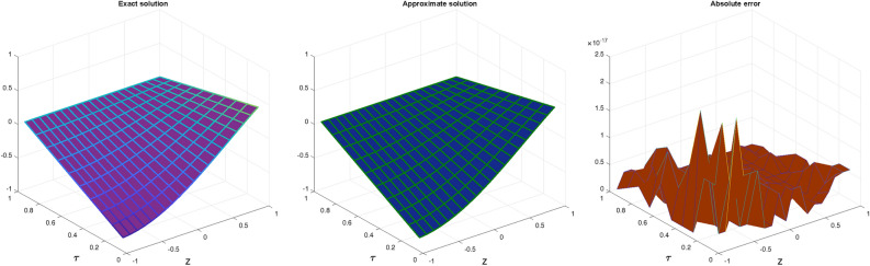
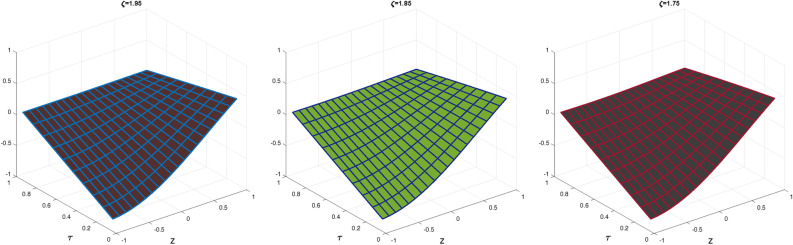
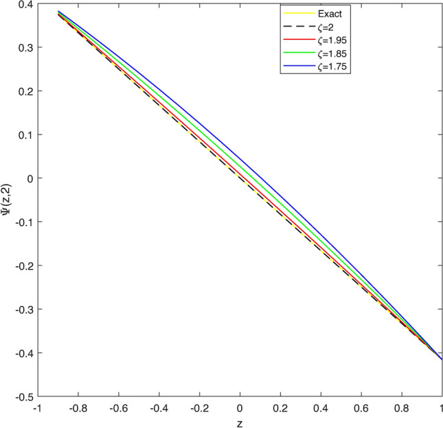
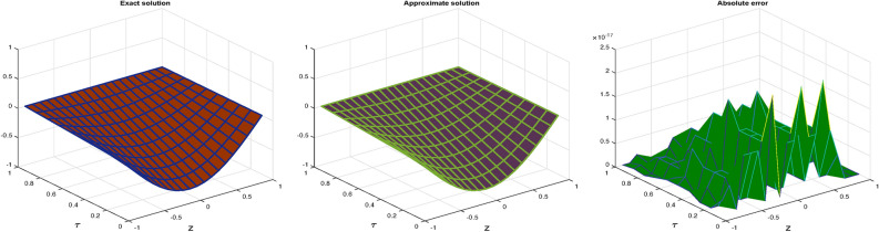
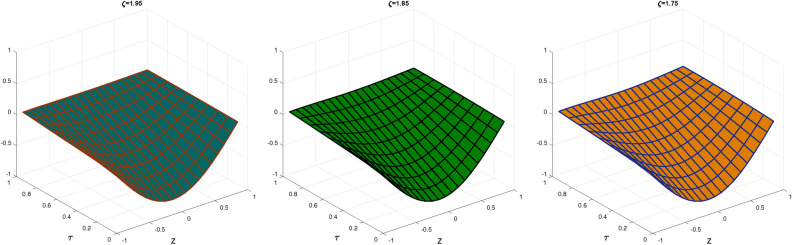
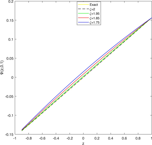
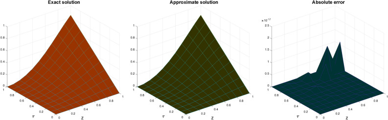
Table 2 display a comparison of error norms for the approximate solution by CBCA-RPSS at \(\zeta =2\) with that Tension spline approach \(O(k^2+k^2h^2+h^2)\) method42, \(O(k^2+k^2h^2+h^4)\) method42, RBF approximation43 and BWCM45 of Problem 2. Figure 4 displays exact solution and CBCA-RPSS solution with its absolute error of Problem 2. Figure 5 expresses the comparison for CBCA-RPSS solution of various fractional-order of \(\zeta\) while Fig. 6 show the behavior of fractional-order \(\zeta\) on CBCA-RPSS solution with exact solution at \(\tau =0.1\) in 2D graph of Problem 2.
Table 2: Comparison of norm errors of CBCA-RPSS with other techniques at \(\zeta =2\) and \(z =0.5\) for problem 2.
| \(\tau\) | \(\mathscr {L}_{2}\ error\) | \(\mathscr {L}_{\infty }\ error\) | RMSE |
|---|---|---|---|
| \(O(k^2+k^2h^2+h^2)\) method42 | |||
| 1 | \(2.71e{-}5\) | \(3.97e{-}6\) | \(2.69e{-}6\) |
| 2 | \(8.97e{-}6\) | \(1.51e{-}6\) | \(8.93e{-}7\) |
| 3 | \(1.49e{-}5\) | \(2.14e{-}6\) | \(1.48e{-}6\) |
| 4 | \(1.05e{-}5\) | \(1.86e{-}6\) | \(1.05e{-}6\) |
| 5 | \(3.36e{-}5\) | \(5.08e{-}6\) | \(3.34e{-}6\) |
| \(O(k^2+k^2h^2+h^4)\) method42 | |||
| 1 | \(2.71e{-}5\) | \(3.97e{-}6\) | \(2.69e{-}6\) |
| 2 | \(8.97e{-}6\) | \(1.51e{-}6\) | \(8.93e{-}7\) |
| 3 | \(1.49e{-}5\) | \(2.14e{-}6\) | \(1.48e{-}6\) |
| 4 | \(1.05e{-}5\) | \(1.86e{-}6\) | \(1.05e{-}6\) |
| 5 | \(3.36e{-}5\) | \(5.08e{-}6\) | \(3.34e{-}6\) |
| BWCM45 | |||
| 1 | \(6.59e{-}16\) | \(3.33e{-}16\) | \(1.98e{-}16\) |
| 2 | \(1.18e{-}15\) | \(5.39e{-}16\) | \(3.58e{-}16\) |
| 3 | \(2.55e{-}14\) | \(1.25e{-}14\) | \(7.70e{-}15\) |
| 4 | \(1.27e{-}13\) | \(6.37e{-}14\) | \(3.85e{-}14\) |
| 5 | \(4.16e{-}13\) | \(2.08e{-}13\) | \(1.25e{-}13\) |
| CBCA-RPSS | |||
| 1 | \(0.00000e+00\) | \(0.00000e+00\) | \(0.00000e+00\) |
| 2 | \(0.00000e+00\) | \(0.00000e+00\) | \(0.00000e+00\) |
| 3 | \(0.00000e+00\) | \(0.00000e+00\) | \(0.00000e+00\) |
| 4 | \(0.00000e+00\) | \(0.00000e+00\) | \(0.00000e+00\) |
| 5 | \(0.00000e+00\) | \(0.00000e+00\) | \(0.00000e+00\) |
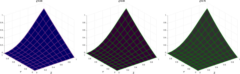
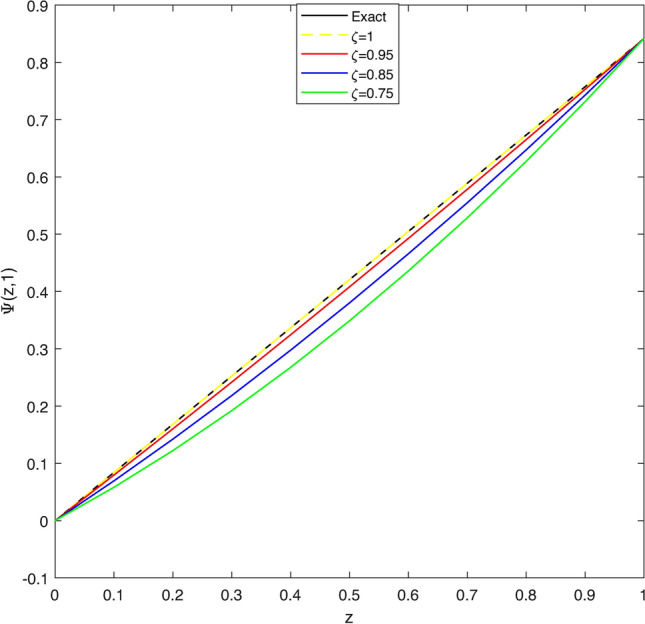
In Table 3, the error norms are reported for \(\zeta =1\) and compared with BWCM45 while in Table 4 show comparison of absolute error of CBCA-RPSS at \(\zeta =1\) and \(z =0.1\) with that BWCM45, ADM with the Bernstein polynomials (BPs)58 and ADM with modified Bernstein polynomials (MBPs)58 of Problem 3. Figure 7 displays exact solution and CBCA-RPSS solution with its absolute error of Problem 3. Figure 8 expresses the comparison for CBCA-RPSS solution of various fractional-order of \(\zeta\) while Fig. 9 demonstrate the behavior of fractional-order \(\zeta\) on CBCA-RPSS solution with exact solution at \(\tau =1\) in 2D graph of Problem 3.
Table 3: Comparison of norm errors of CBCA-RPSS with other techniques at \(\zeta =1\) and \(z =0.1\) for problem 3.
| \(\tau\) | \(\mathscr {L}_{2}\ error\) | \(\mathscr {L}_{\infty }\ error\) | RMSE |
|---|---|---|---|
| BWCM45 | |||
| 1 | \(2.6161e{-}12\) | \(1.0940e{-}12\) | \(7.8878e{-}13\) |
| 2 | \(8.1931e{-}10\) | \(3.9878e{-}10\) | \(2.4703e{-}10\) |
| 3 | \(7.4899e{-}9\) | \(3.7339e{-}9\) | \(2.2582e{-}9\) |
| 4 | \(3.0534e{-}8\) | \(1.5343e{-}8\) | \(9.2065e{-}9\) |
| 5 | \(8.5980e -8\) | \(4.3370e{-}8\) | \(2.5923e{-}8\) |
| CBCA-RPSS | |||
| 1 | \(0.00000e+00\) | \(0.00000e+00\) | \(0.00000e+00\) |
| 2 | \(0.00000e+00\) | \(0.00000e+00\) | \(0.00000e+00\) |
| 3 | \(0.00000e +00\) | \(0.00000e+00\) | \(0.00000e+00\) |
| 4 | \(0.00000e+00\) | \(0.00000e+00\) | \(0.00000 \ e+00\) |
| 5 | \(1.93948e{-}19\) | \(1.73472e{-}18\) | \(8.26059e{-}20\) |
Table 4: Comparison of absolute error of CBCA-RPSS with other methods at \(\zeta =1\) and \(z =0.1\) for problem 3.
| \(\tau\) | \(\mathscr {A}_1\) | \(\mathscr {A}_2\) | \(\mathscr {A}_3\) | \(\mathscr {A}_4\) |
|---|---|---|---|---|
| 0 | 0.00000e+00 | 0.00000e+00 | 0.00000e+00 | 0.00000e+00 |
| 0.1 | \(5.5121e{-}6\) | \(4.1490e{-}6\) | \(1.4528e{-}16\) | 0.00000e+00 |
| 0.2 | \(3.4011e{-}5\) | \(1.8495e{-}6\) | \(3.9161e{-}15\) | 0.00000e+00 |
| 0.3 | \(8.8513 e{-}5\) | \(2.8381e{-}5\) | \(1.6276e{-}14\) | 0.00000e+00 |
| 0.4 | \(1.4044e{-}5\) | \(9.1215 e{-}5\) | \(3.8899e{-}14\) | 0.00000e+00 |
| 0.5 | \(1.2560 e{-}4\) | \(1.6204 e{-}4\) | \(7.0159e{-}14\) | 0.00000e+00 |
| 0.6 | \(4.2509 e{-}5\) | \(1.8804e{-}4\) | \(1.0514 e{-}13\) | 0.00000e+00 |
| 0.7 | \(4.3607e{-}4\) | \(1.0861e{-}4\) | \(1.3563e{-}13\) | \(6.93889e{-}18\) |
| 0.8 | \(1.0501 e{-}3\) | \(1.0202 e{-}4\) | \(1.5012e{-}13\) | 0.00000e+00 |
| 0.9 | \(1.7188e{-}3\) | \(3.7522e{-}4\) | \(1.3385e{-}13\) | 0.00000e+00 |
| 1 | \(2.0247e{-}3\) | \(4.8632e{-}4\) | \(6.8667e{-}14\) | 0.00000e+00 |
\(\mathscr {A}_1\) absolute error by ADM with BPs58
\(\mathscr {A}_2\) absolute error by
ADM with MBPs58
\(\mathscr {A}_3\) absolute error by BWCM45
\(\mathscr {A}_4\) absolute error by CBCA-RPSS
Concluding remarks
In this paper, CBCA-RPSS was successfully used to obtain an approximate solution for non-linear time-fractional KGP. First, by utilizing confluent Bernoulli polynomial and their properties the non-linear time-fractional KGP is reduced into a system of FODEs. Secondly, the RPSS is used to solve these system of equations with helping of the given initial and boundary conditions. We derived some theories of convergence, uniqueness and error analysis of proposed method. Finally, the comparisons of results abtained by CBCA-RPSS were performed and found that it is very computationally accurate than other existing techniques in literature42–45,58. Also, this comparisons shows that present method is very straightforward, simple, accurate and can be applied to solve nonlinear PDE problems that arise in engineering problems and complex phenomena.
References
- NH Sweilam, MM Abou Hasan, D Baleanu. New studies for general fractional financial models of awareness and trial advertising decisions. Chaos Solitons Fract., 2017. [DOI]
- BJ West, M Turalska, P Grigolini. Fractional calculus ties the microscopic and macroscopic scales of complex network dynamics. New J. Phys., 2015. [DOI]
- A Esen, TA Sulaiman, H Bulut, HM Baskonus. Optical solitons to the space-time fractional (1+ 1)-dimensional coupled non-linear Schrödinger equation. Optik, 2018. [DOI]
- HM Ali, H Ahmad, S Askar, IG Ameen. Efficient approaches for solving systems of nonlinear time-fractional partial differential equations. Fractal Fract., 2022. [DOI]
- 5.Podlubny, I. Fractional differential equations, mathematics in science and engineering. (1999).
- HAA El-Saka El-Saka, AAM Arafa, MI Gouda. Dynamical analysis of a fractional SIRS model on homogenous networks. Adv. Differ. Equ., 2019
- AAM Arafa, M Khalil, A Sayed. A non-integer variable order mathematical model of human immunodeficiency virus and malaria coinfection with time delay. Complexity, 2019. [DOI]
- AMA El-Sayed, SZ Rida, AAM Arafa. On the solutions of the generalized reaction-diffusion model for bacterial colony. Acta Appl. Math., 2010. [DOI]
- IG Ameen, RO Ahmed Taie, HM Ali. Two effective methods for solving nonlinear coupled time-fractional Schrodinger equations. Alex. Eng. J., 2023. [DOI]
- SR Khirsariya, SB Rao, GS Hathiwala. Investigation of fractional diabetes model involving glucose-insulin alliance scheme. Int. J. Dyn. Control, 2024. [DOI]
- Y Jiang, J Ma. High-order finite element methods for time-fractional partial differential equations. J. Comput. Appl. Math., 2011. [DOI]
- NA Shah, X Wang, H Qi, S Wang, A Hajizadeh. Transient electro-osmotic slip flow of an oldroyd-B fluid with time-fractional Caputo-Fabrizio derivative. J. Appl. Comput. Mech., 2019
- 13.Nawaz Khan, M., Ahmad, I. & Ahmad, H. A radial basis function collocation method for space-dependent inverse heat problems. J. Appl. Comput. Mech. (2020).
- JP Chauhan, SR Khirsariya. A semi-analytic method to solve nonlinear differential equations with arbitrary order. Results Control Optim., 2023. [DOI]
- AA Arafa, AMS Hagag. A new analytic solution of fractional coupled Ramani equation. Chin. J. Phys., 2019. [DOI]
- 16.Khirsariya, S. R. & Rao, S. B. On the semi-analytic technique to deal with nonlinear fractional differential equations. J. Appl. Math. Comput. Mech.22(1) (2023).
- 17.Khater, M., Lu, D. & Attia, R. A. Dispersive long wave of non-linear fractional Wu-Zhang system via a modified auxiliary equation method. AIP Adv.9(2), (2019).
- SR Khirsariya, SB Rao. Solution of fractional Sawada-Kotera-Ito equation using Caputo and Atangana-Baleanu derivatives. Math. Methods Appl. Sci., 2023. [DOI]
- SR Khirsariya, SB Rao, JP Chauhan. A novel hybrid technique to obtain the solution of generalized fractional-order differential equations. Math. Comput. Simul., 2023. [DOI]
- IG Ameen, MK Elboree, RO Ahmed Taie. Traveling wave solutions to the nonlinear space-time fractional extended KdV equation via efficient analytical approaches. Ale. Eng. J., 2023. [DOI]
- JP Chauhan, SR Khirsariya, GS Hathiwala, M Biswas Hathiwala. New analytical technique to solve fractional-order Sharma-Tasso-Olver differential equation using Caputo and Atangana-Baleanu derivative operators. J. Appl. Anal., 2024. [DOI]
- OA Arqub. Series solution of fuzzy differential equations under strongly generalized differentiability. J. Adv. Res. Appl. Math., 2013. [DOI]
- A El-Ajou, OA Arqub, S Momani. Approximate analytical solution of the non-linear fractional KdV-Burgers equation: a new iterative algorithm. J. Comput. Phys., 2015. [DOI]
- H Khan, Q Khan, P Kumam, F Tchier, S Ahmed, G Singh, K Sitthithakerngkiet. The fractional view analysis of the Navier-Stokes equations within Caputo operator. Chaos Solitons Fract. X., 2022. [DOI]
- DG Prakasha, P Veeresha, HM Baskonus. Residual power series method for fractional Swift-Hohenberg equation. Fractal Fract., 2019. [DOI]
- 26.Al-Smadi, M., Al-Omari, S., Karaca, Y. & Momani, S. Effective analytical computational technique for conformable time-fractional non-linear Gardner equation and Cahn-Hilliard equations of eourth and sixth order emerging in dispersive media. J. Funct. Spaces. 2022 (2022).
- SZ Rida, AA Arafa, HS Hussein, IG Ameen, MM Mostafa. Spectral shifted Chebyshev collocation technique with residual power series algorithm for time fractional problems. Sci. Rep., 2024. [DOI | PubMed]
- S Khirsariya, S Rao, J Chauhan. Semi-analytic solution of time-fractional Korteweg-de Vries equation using fractional residual power series method. Results Nonlinear Anal., 2022. [DOI]
- SR Khirsariya, JP Chauhan, SB Rao. A robust computational analysis of residual power series involving general transform to solve fractional differential equations. Math. Comput. Simul., 2024. [DOI]
- S Khirsariya, S Rao, J Chauhan. Solution of fractional modified Kawahara equation: a semi-analytic approach. Math. Appl. Sci. Eng., 2023. [DOI]
- 31.Sassaman, R. & Biswas, A. Soliton solution of the generalized Klein-Gordon equation by semi-inverse variational principle. Math. Eng. Sci. Aerospace (MESA). 2(1), (2011).
- 32.Sassaman, R. & Biswas, A. 1-soliton solution of the perturbed Klein-Gordon equation. (2011).
- PJ Caudrey, JC Eilbeck, JD Gibbon. The sine-Gordon equation as a model classical field theory. Il Nuovo Cimento B., 1975. [DOI]
- AM Wazwaz. New travelling wave solutions to the Boussinesq and the Klein-Gordon equations. Commun. Nonlinear Sci. Numer. Simul., 2008. [DOI]
- AM Wazwaz. Compactons, solitons and periodic solutions for some forms of nonlinear Klein-Gordon equations. Chaos Solitons Fract., 2006. [DOI]
- M Song, Z Liu, E Zerrad, A Biswas. Singular soliton solution and bifurcation analysis of Klein-Gordon equation with power law nonlinearity. Front. Math. China., 2013. [DOI]
- M Yaseen, M Abbas, B Ahmad. Numerical simulation of the non-linear generalized time-fractional Klein-Gordon equation using cubic trigonometric B-spline functions. Math. Methods Appl. Sci., 2021. [DOI]
- G Hariharan. Wavelet method for a class of fractional Klein-Gordon equations. J. Comput. Nonlinear Dynam., 2013. [DOI]
- SA Khuri, A Sayfy. A spline collocation approach for the numerical solution of a generalized non-linear Klein-Gordon equation. Appl. Math. Comput., 2010
- AA Arafa. Analytical solutions for non-linear fractional physical problems via natural homotopy perturbation method. Int. J. Appl. Comput. Math., 2021. [DOI]
- MSH Chowdhury, I Hashim. Application of homotopy-perturbation method to Klein-Gordon and sine-Gordon equations. Chaos Solitons Fract., 2009. [DOI]
- J Rashidinia, R Mohammadi. Tension spline approach for the numerical solution of non-linear Klein-Gordon equation. Comput. Phys. Commun., 2010. [DOI]
- M Dehghan, A Shokri. Numerical solution of the non-linear Klein-Gordon equation using radial basis functions. J. Comput. Appl. Math., 2009. [DOI]
- S Kumbinarasaiah, HS Ramane, KS Pise, G Hariharan. Numerical solution for non-linear Klein-Gordon equation via operational matrix by clique polynomial of complete graphs. Int. J. Appl. Comput. Math., 2021. [DOI]
- S Kumbinarasaiah, M Mulimani. Bernoulli wavelets numerical approach for the non-linear Klei-Gordon and Benjami-Bona-Mahony equation. Int. J. Appl. Comput. Math., 2023. [DOI]
- AM Nagy. Numerical solution of time-fractional non-linear Klein-Gordon equation using Sinc-Chebyshev collocation method. Appl. Math. Comput., 2017
- RM Ganji, H Jafari, M Kgarose, A Mohammadi. Numerical solutions of time-fractional Klein-Gordon equations by clique polynomials. Alex. Eng. J., 2021. [DOI]
- Y Zhang. Time-fractional Klein-Gordon equation: formulation and solution using variational methods. WSEAS Trans. Math., 2016
- 49.Raza, N., Butt, A. R., Javid, A.: Approximate solution of non-linear klein-Gordon equation using sobolev gradients. J. Funct. Spaces.2016 (2016).
- MG Hafez, MN Alam, MA Akbar. Exact traveling wave solutions to the Klein-Gordon equation using the novel expansion method. Results Phys., 2014. [DOI]
- D Kumar, J Singh, S Kumar. Numerical computation of Klein-Gordon equations arising in quantum field theory by using homotopy analysis transform method. Alex. Eng. J., 2014. [DOI]
- 52.Kilbas, A. A., Marichev, O. I. & Samko, S. G. Fractional integrals and derivatives (theory and applications). (1993).
- MA Bayrak, A Demir. A new approach for space-time fractional partial differential equations by residual power series method. Appl. Math. Comput., 2018
- A Pourdarvish, K Sayevand, I Masti, S Kumar. Orthonormal Bernoulli polynomials for solving a class of two dimensional stochastic Volterra-Fredholm integral equations. Int. J. Appl. Comput. Math., 2022. [DOI | PubMed]
- MA Ozarslan, B Cekim. Confluent Appell polynomials. J. Comput. Appl. Math., 2023. [DOI]
- K Pavani, K Raghavendar, K Aruna. Solitary wave solutions of the time fractional Benjamin Bona Mahony Burger equation. Sci. Rep., 2024. [DOI | PubMed]
- MK Iqbal, M Abbas, B Zafar. New quartic B-spline approximations for numerical solution of fourth order singular boundary value problems. Punjab Univ. J. Math., 2020
- 58.Qasim, A.F. & AL-Rawi, E.S. Adomian decomposition method with modified Bernstein polynomials for solving ordinary and partial differential equations. J. Appl. Math.2018, (2018).