Most large structural variants in cancer genomes can be detected without long reads

Article type: Research Article

Keywords: Genomics, Computational biology and bioinformatics, Genome assembly algorithms

Authors: Zi-Ning Choo, Julie M. Behr, Aditya Deshpande, Kevin Hadi, Xiaotong Yao, Huasong Tian, Kaori Takai, George Zakusilo, Joel Rosiene ⚬, Arnaud Da Cruz Paula ⚬, Britta Weigelt ⚬, Jeremy Setton, Nadeem Riaz ⚬, Simon N. Powell ⚬, Klaus Busam ⚬, Alexander N. Shoushtari, Charlotte Ariyan, Jorge Reis-Filho ⚬, Titia de Lange ⚬, Marcin Imieliński ⚬

Affiliations: https://ror.org/05wf2ga96grid.429884.b0000 0004 1791 0895New York Genome Center, New York, NY USA; https://ror.org/02r109517grid.471410.70000 0001 2179 7643Department of Pathology and Laboratory Medicine, Weill Cornell Medicine, New York, NY USA; https://ror.org/02r109517grid.471410.70000 0001 2179 7643Tri-institutional MD PhD Program, Weill Cornell Medicine, New York, NY USA; https://ror.org/02r109517grid.471410.70000 0001 2179 7643Physiology and Biophysics PhD Program, Weill Cornell Medicine, New York, NY USA; grid.517640.1Tri-institutional PhD Program in Computational Biology and Medicine, New York, NY USA; grid.137628.90000 0004 1936 8753Perlmutter Cancer Center, NYU Grossman School of Medicine, New York, NY USA; https://ror.org/0420db125grid.134907.80000 0001 2166 1519Laboratory of Cell Biology and Genetics, Rockefeller University, New York, NY USA; https://ror.org/02yrq0923grid.51462.340000 0001 2171 9952Memorial Sloan Kettering Cancer Center, New York, NY USA; grid.137628.90000 0004 1936 8753Department of Pathology, NYU Grossman School of Medicine, New York, NY USA

License: © The Author(s) 2023 CC BY 4.0 Open Access This article is licensed under a Creative Commons Attribution 4.0 International License, which permits use, sharing, adaptation, distribution and reproduction in any medium or format, as long as you give appropriate credit to the original author(s) and the source, provide a link to the Creative Commons license, and indicate if changes were made. The images or other third party material in this article are included in the article’s Creative Commons license, unless indicated otherwise in a credit line to the material. If material is not included in the article’s Creative Commons license and your intended use is not permitted by statutory regulation or exceeds the permitted use, you will need to obtain permission directly from the copyright holder. To view a copy of this license, visit http://creativecommons.org/licenses/by/4.0/.

Article links: DOI: 10.1038/s41588-023-01540-6  |  PubMed: 37945902  |  PMC: PMC10703688

Relevance: Moderate: mentioned 3+ times in text

Full text: PDF (525 KB)

Main

It is widely thought that short-read sequencing (SRS), which usually generates ≤150-bp reads, has limited sensitivity for mapping cancer structural variants (SVs; copy number (CN) alterations and rearrangements) owing to the many homologous sequences in the human genome¹. Indeed, more than two-thirds of the human genome consists of repetitive sequences², including transposable elements, satellites and telomeres. SVs that rearrange long homologous repeats are likely to be missed by SRS.

Cancer whole-genome profiling efforts have been carried out almost exclusively with SRS^3–5. Hence, little is known about the nature and burden of cancer SVs missed by SRS. While most cancer rearrangements detected with SRS have negligible breakend homology^3,6–8, it is also unknown whether additional homologous recombination-driven mutational processes govern the evolution of rearrangements that are undetectable by SRS^1,9.

Owing to mass balance, every copy of every segment in a genome must either have both a left and right neighbor or reside at a chromosome end. Because rearrangements appose previously distant segment ends to create new junctions, CN alterations and rearrangements are physically coupled in the cancer genome; most CN alterations involve a rearrangement, and many rearrangements are associated with a CN alteration^4,10–13.

This coupling can be formalized as ‘junction balance constraints’ on a graph of genomic segments and their junctions⁴ (Fig. 1a). These constraints state that the CN of each genomic segment is equal to the CN of the junctions connecting to its left and right sides. Enforcing these and other constraints within a statistical model enables the inference of balanced genome graphs and high-fidelity CN profiles from whole-genome SRS data, as shown with our previously published JaBbA (v0.1) algorithm⁴.

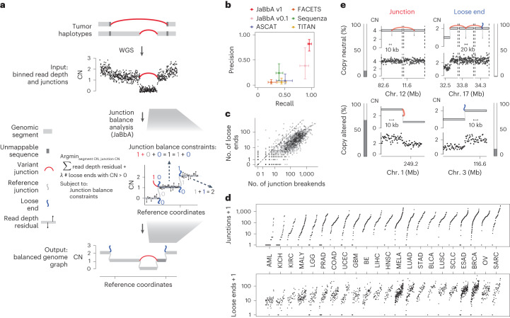
JaBbA’s statistical model allows for ‘loose ends’, which are ‘placeholder’ adjacencies that allow the graph to satisfy junction balance while violating mass balance (Fig. 1a). Loose ends allow JaBbA to be robust to missing data but also represent hypotheses about unmapped junctions. We reasoned that analysis of loose ends in JaBbA could be used to test the completeness of cancer genome reconstructions from SRS and assess the nature of missing SVs in SRS profiles. In particular, we focused on large (>10-kb) SVs that give rise to clonal chromosomal alterations in cancers (referred to as SVs below for brevity, unless otherwise qualified). Our goal was to understand the impact of mutational processes that specifically rearrange repetitive sequences, including aberrant homologous recombination, on cancer chromosomal structure.

Results

JaBbA v1 outperforms previous CN algorithms

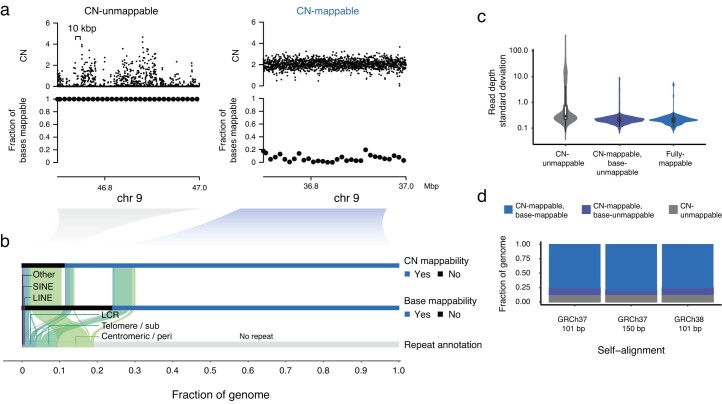
We enhanced our previous JaBbA (v0.1; ref. ⁴) model with several methodological innovations to increase robustness to read depth waviness, improve algorithm convergence and enforce junction balance for allele-specific as well as total CN (Extended Data Fig. 1a–d and Methods). We also rigorously defined ‘CN-unmappable’ regions in the genome as positions surrounded by >90% repetitive bases in their 1-kb vicinity. CN-unmappable regions accounted for 13% of the genome (across read lengths and genome builds), primarily comprised regions in or around telomeres and centromeres, and showed high variance in read depth across a panel of diploid normal samples (Methods and Extended Data Fig. 2). We then limited analysis with the updated model (JaBbA v1) to the 87% of the human genome that was CN-mappable.

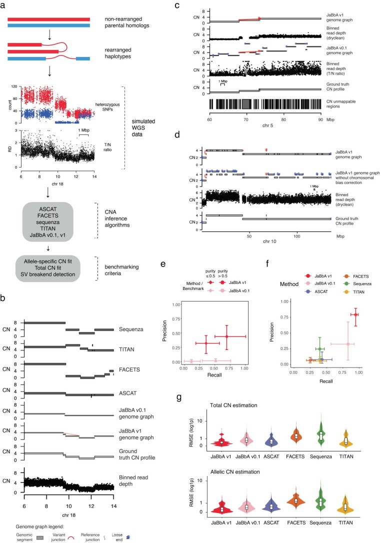
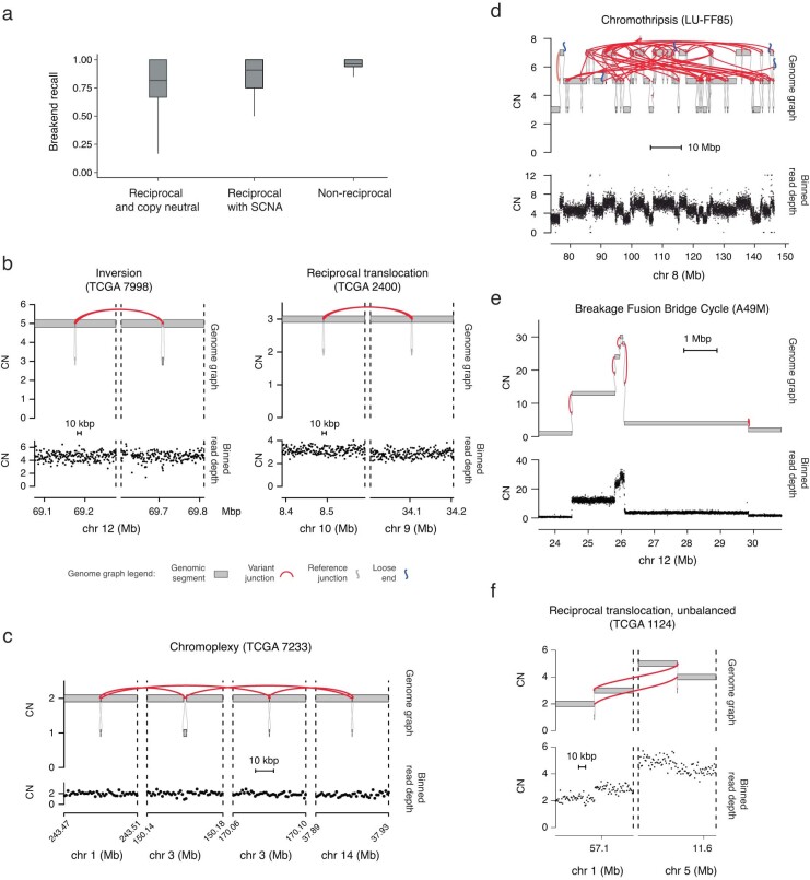
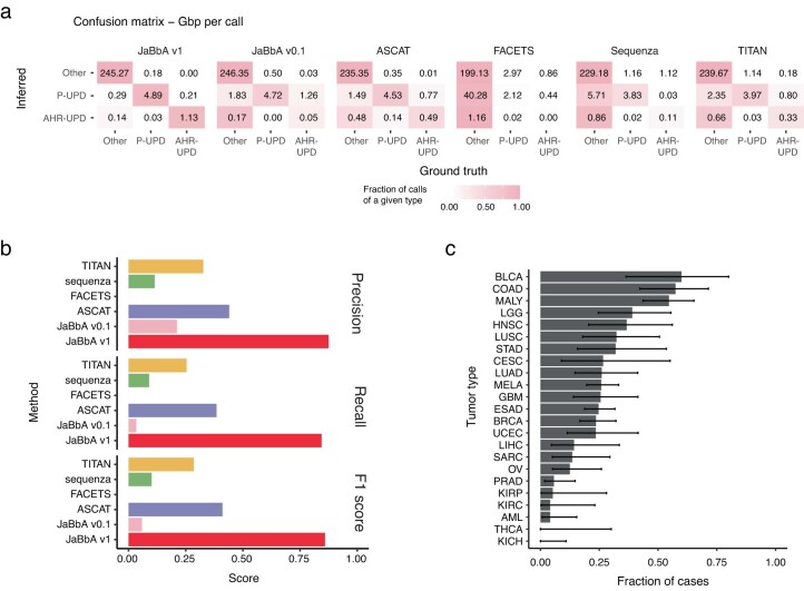
To assess the accuracy of JaBbA v1 for SV breakend detection in CN-mappable regions, we simulated 500 SRS whole-genome profiles comprising binned (1-kb) read depth, single nucleotide polymorphism (SNP) read counts and SV junctions (Extended Data Fig. 3a–d and Methods). In these simulations, JaBbA v1 loose ends showed substantially higher precision (median of 43% versus 5%) and recall (median of 70% versus 54%) than JaBbA v0.1 loose ends for missing CN-mappable SVs in high-purity (>0.5) cancer genomes (Extended Data Fig. 3e). JaBbA v1 also showed markedly improved accuracy for overall CN-mappable SV breakend inference relative to both JaBbA v0.1 and four state-of-the-art cancer CN inference algorithms (ASCAT¹⁴, TITAN¹⁵, Sequenza¹⁶ and FACETS¹⁷) (Extended Data Fig. 3f), particularly for high-purity samples (median precision of 82% (68–91%) and median recall of 96% (93–100%), with the interquartile range (IQR) in parentheses) (Fig. 1b). JaBbA v1 also accurately estimated both total and allelic CN (Extended Data Fig. 3g), suggesting that JaBbA v1 is a state-of-the-art algorithm for the inference of CN and missing SVs in cancer genomes.

Pan-cancer landscape of loose ends

We next applied JaBbA v1 to 1,330 high-purity tumor and matched normal SRS profiles previously analyzed in Hadi et al.⁴ (see Methods for details), identifying 154,322 (clonal and somatic) junctions (median of 63 per tumor sample) and 48,835 somatic loose ends (median of 21 per tumor sample). The somatic loose end burden per sample varied across a 200-fold range and was correlated (Spearman R² = 0.68) with the junction burden (Fig. 1c,d).

Junction breakends may be reciprocal, meaning that they are near (within 10 kb) of another breakend with opposite orientation. Reciprocal breakends are usually copy-neutral (Fig. 1e, top left) which makes them difficult to detect through classic CN analyses. JaBbA’s bookkeeping of mass balance across segments and junctions enables sensitive detection of reciprocal and nonreciprocal SVs at both copy-neutral and copy-altered genomic regions (Extended Data Fig. 4a–e). Across cancer, we found that most (85%) cancer junctions were both nonreciprocal and copy-altered (Fig. 1e, bottom left). Such junctions can arise from inherently nonreciprocal SVs, such as simple deletions, or begin as reciprocal translocations that undergo subsequent loss or gain of one of the derivative alleles (Extended Data Fig. 4f). Like somatic junction breakends, somatic loose ends were predominantly (92%) copy-altered (Fig. 1e, bottom right), although copy-neutral loose ends were also identified (Fig. 1e, top right). Taken together, these results suggest that loose ends arise by breakage and repair mutational processes similar to those generating junction breakends.

Loose ends harbor repetitive and foreign sequences

To study the sequence context around loose ends, we defined a canonical axis originating at the loose end with coordinates increasing along the DNA strand whose 3′ terminus matches the side of a segment on which a loose end is found, which we refer to as the loose end’s ‘forward’ strand (Fig. 2a). We next asked whether loose ends occurred preferentially at reference sequence repeats. Indeed, we found that unmappable bases were enriched near loose ends, most frequently LINE elements (Fig. 2b and Extended Data Fig. 5a). We next reasoned that some loose ends would result from the somatic fusion of mappable bases to unalignable sequences. Confirming this, we found a tumor-specific enrichment of repetitive and foreign sequences, including satellite and viral sequences, mated to reads on the forward (but not reverse) strand of somatic loose ends (Fig. 2c and Extended Data Fig. 5b).

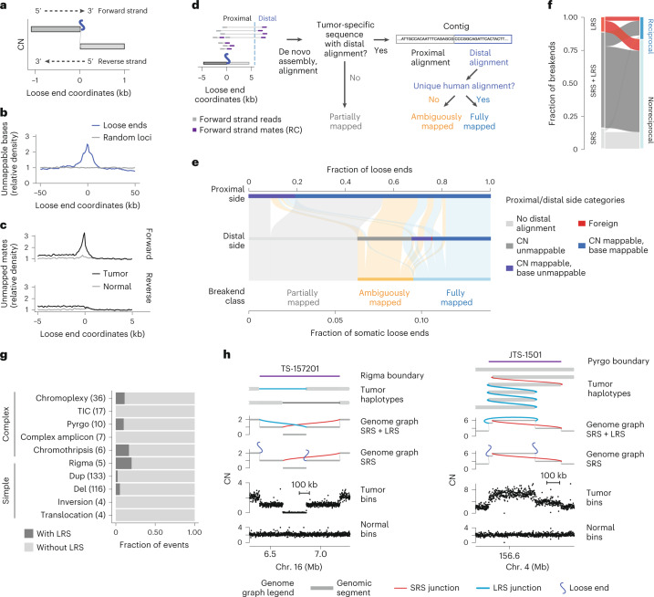
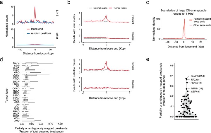
To identify distinct classes of repetitive SVs missing from SRS whole-genome profiles, we systematically classified tumor-specific sequences fused to each somatic loose end through assembly or consensus alignment (Fig. 2d and Methods). Overall, 55% of somatic loose ends showed evidence of tumor-specific fusion to a distal sequence. For over half of these (33% of somatic loose ends), the distal sequence aligned uniquely, indicating that these were fully mapped breakends missed by the initial junction caller (Fig. 2e) (SvAbA¹⁸). In 23% of somatic loose ends (3% of detected breakends), the distal sequence was repetitive or foreign and could not be unambiguously placed on any reference (ambiguously mapped breakends; Fig. 2e). Finally, 45% of somatic loose ends (6% of detected breakends) did not map to any distal location (partially mapped breakends; Fig. 2e). Notably, partially mapped breakends were enriched in boundaries of large (>1-Mb) CN-unmappable regions (odds ratio (OR) = 3.8; P < 2 × 10⁻¹⁶) (Extended Data Fig. 5c), indicating that some represented CN changes shifted away from a CN-unmappable SV breakend (for example, centromeric breakends causing arm-level chromosomal changes).

Combining fully mapped breakends across both loose ends and junctions indicated that 91% of JaBbA v1 breakends could be uniquely mapped. Notably, the fraction of partially or ambiguously mapped breakends did not vary substantially across cancer types (Extended Data Fig. 5d; range of 5–33%) or established cancer drivers (Extended Data Fig. 5e; range of 0–38%), although we observed tumor types (for example, acute myeloid leukemia) and cancer genes (SMARCB1, TSC2 and FGFR3) with higher (>25%) fractional burdens. Given the estimated recall of JaBbA v1 (~96%), these results suggest that 87% of cancer SVs in the 87% of the genome that is CN-mappable can be fully resolved by SRS.

Long-molecule validation

To orthogonally assess these SRS-derived estimates of missing somatic SVs, we profiled the whole genomes of 11 melanoma (n = 10) and breast cancer (n = 1) tumor samples and their matched normal tissues with both SRS and Oxford Nanopore Technologies long-read sequencing (LRS; median read N50 of 11 kb; median coverage of 73× and 32× for tumor and normal samples, respectively). After calling large (>10-kb) somatic SVs in CN-mappable regions (Methods), we found a strong overlap (87%, 7,258 breakends) between LRS and SRS breakends, including 77% overlap with fully mapped SRS breakends (Fig. 2f). The majority of junction calls identified by either platform had local read depth changes that were consistent with breakend topology; reciprocal breakends were copy-neutral, whereas nonreciprocal breakends showed a CN drop along their forward strand (Extended Data Fig. 6a). This analysis along with manual inspection of long and short read support at inidivudal junctions (Extended Data Fig. 6b) suggested that both SRS-only and LRS-only junctions comprise largely true positives; combining SRS and LRS breakend counts suggests that SRS missed ~12% of breakends. This result is consistent with our simulation-based estimate of recall (Fig. 1b and Extended Data Fig. 3f). Notably, we found a similar proportion of reciprocal and non-reciprocal breakends among those detected and missed by SRS (Fig. 2f), indicating that reciprocal and copy-neutral breakends do not comprise the bulk of missed structural variation in cancer genomes. These results confirm our SRS findings that most cancer SVs are nonreciprocal and copy-altered (Fig. 1e).

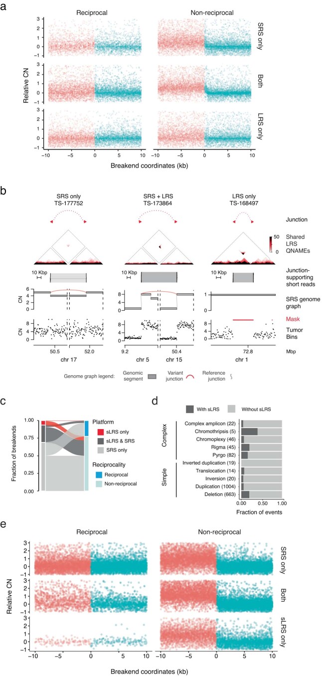
We next asked whether LRS improved SV event detection, which relies on the recognition of high-order patterns across multiple junctions^3,4. Although LRS did not help identify many additional simple or complex events relative to SRS (Fig. 2g), LRS junctions also resolved breakends at complex SVs found by SRS, including for chromothripsis, pyrgo, rigma and templated insertion chains^3,4. The incorporation of LRS junctions enabled more complete haplotype reconstruction at loci where SRS found loose ends (Fig. 2h).

As additional validation of our results, we analyzed 27 high-purity (purity of >0.5) breast cancer and matched normal samples with both SRS and synthetic LRS (sLRS) whole-genome profiles (10x Genomics linked reads, median N50 molecule length of 23 kb, median coverage of 173× and 98× in tumor and normal samples, respectively; Methods)¹⁹. Similar to LRS, most sLRS SV calls (Methods) overlapped with SRS breakends, showed concordant patterns of reciprocality and CN change, and yielded similar complex SV calls in sLRS junction-augmented genome graphs (Extended Data Fig. 6c–e). These breast cancer and melanoma LRS and sLRS results are consistent with our pan-cancer finding that SRS captures most large cancer SVs in CN-mappable regions.

Loose ends reveal neotelomeres

We next sought to investigate specific mutational processes engendering loose ends. We observed that a fraction (4.8%) of ambiguously mapped loose ends (0.01% of all breakends) were fused to telomere repeats, as evidenced by telomere repeat-positive sequences mated to reads on the positive loose end strand (Fig. 3a). We refer to these breakends as telomere repeat-positive loose ends and surmised that they might represent neotelomeres, telomere-stabilized chromosome ends at previously interstitial genomic loci.

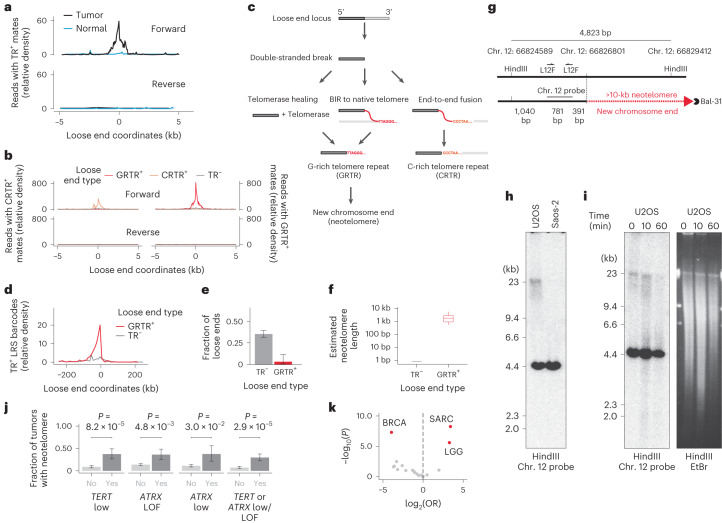
Telomere repeat-positive mates were found on the forward strand of telomere repeat-positive loose ends, but not on the reverse strand or in matched normal samples (Fig. 3a), indicating that these were neither telomere insertions^20,21 nor constitutional neotelomeres^22,23. Deeper analysis of telomere repeats at loose ends revealed strong strand bias, with loose ends harboring either G-rich (GRTR) or C-rich (CRTR) repeats but not both (Fig. 3b). The GRTR pattern is consistent with a neotelomere, whereas the CRTR pattern is consistent with the fusion of an interstitial sequence to a native chromosome end (Fig. 3c, right). The predominance of the GRTR pattern among telomere repeat-positive loose ends, in combination with the tumor specificity and forward strand bias, suggested that somatic neotelomeres are frequent in cancer.

To better assess sequences fused to GRTR⁺ loose ends, we profiled three cancer cell lines (U2OS, NCI-H526 and NCI-H838) with sLRS (Methods). We found telomere repeat-positive linked reads within 5 kb of 26 of 31 GRTR⁺ loose ends (83.8%) (Methods). Telomere repeat-positive linked reads were found up to 50 kb upstream of each GRTR⁺ loose end, indicating power to map distal fusion partners at these loci (Fig. 3d). In contrast to sLRS junctions and telomere repeat-negative loose ends, linked reads at GRTR⁺ loose ends rarely (<1.5%) mapped to distant chromosomal locations, consistent with new chromosome ends (Fig. 3e). Quantitative analysis of repeat counts at linked reads mapping to these loci (Methods) revealed 2.4 ± 1.3 (s.d.) kb of telomere repeats per GRTR⁺ locus, in line with previous estimates of native cancer telomere lengths²⁰ (Fig. 3f).

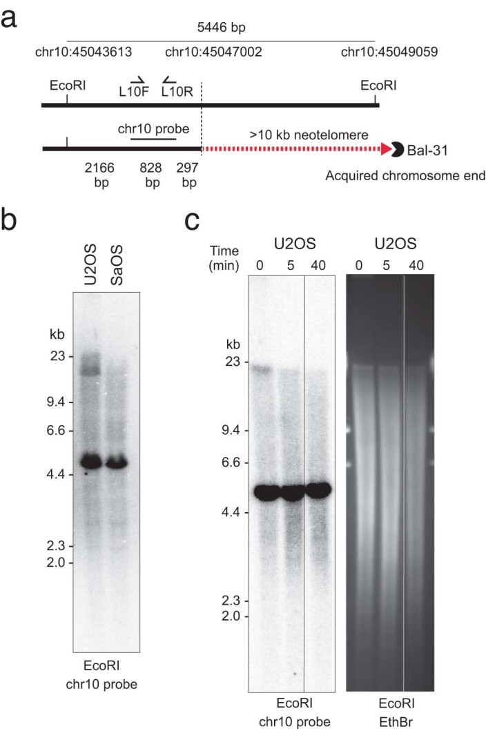
To confirm that GRTR⁺ loose ends were indeed chromosome ends, we performed Southern blot analysis on restriction-digested U2OS and control (Saos-2) genomic DNA using radiolabeled probes against two U2OS GRTR⁺ loose ends. At each locus (Fig. 3g and Extended Data Fig. 7a), we found a small (<5-kb) band consistent with an unaltered reference allele and a longer U2OS-specific diffuse band consistent with a neotelomere (Fig. 3h and Extended Data Fig. 7b). To further investigate the nature of these nonreference bands, we subjected intact genomic DNA to exonuclease (Bal-31) digestion²⁴. The U2OS-specific (but not wild-type) bands disappeared with prolonged exonuclease exposure (Fig. 3i and Extended Data Fig. 7c), consistent with their origin at a chromosome end. These results establish these two U2OS GRTR⁺ loose ends as bona fide neotelomeres.

We next hypothesized that telomerase-mediated healing of double-stranded DNA breaks might give rise to neotelomeres (Fig. 3c, left)²⁵. However, neotelomeres were not found more frequently in tumors that amplified TERT or expressed it at high levels (CN > 2 ploidy, expression z score > 2). Instead, neotelomeres were enriched in samples with low or negligible TERT expression (reads per kilobase per million mapped reads (RPKM) = 0) (Fig. 3j). Tumors that lack telomerase may activate the alternative lengthening of telomeres (ALT) pathway, a break-induced replication (BIR) process (Fig. 3c, middle) suppressed by ATRX²⁶. Indeed, we found that neotelomeres were significantly more common in tumors harboring truncating mutations in ATRX than in ATRX-wild-type cancers (Fig. 3j). Furthermore, we found that several ALT-associated cancers, including sarcomas (18%; OR = 6.47; P = 1.95 × 10⁻⁵) and low-grade gliomas (12.3%; OR = 3.92; P = 4.1 × 10⁻³), had the highest rate of GRTR⁺ loose ends relative to other tumor types (Fig. 3k). These results indicate that GRTR⁺ loose ends and neotelomeres may be a new hallmark of the ALT phenotype.

Loose ends link viral integration to amplicon formation

Surveying additional mutational processes engendering loose ends, we found ambiguously mapped somatic breakends fused to viral sequences, indicating junctional viral integration at large SVs (Extended Data Fig. 8a). While the integration of viral sequences into otherwise unrearranged loci (Extended Data Fig. 8a, left) has been widely studied in cancer^27,28, the role of viruses in causing chromosomal-scale SVs (Extended Data Fig. 8a, right) has been a topic of only recent interest^29–31. Somatic loose ends harboring tumor-specific viral sequence (viral loose ends) were rare overall (~1% of cancers), although enriched in cancer types with viral etiology in our dataset⁴: cervical squamous cell carcinoma (CESC; 32%), liver hepatocellular carcinoma (LIHC; 13%) and head and neck squamous cell carcinoma (HNSC; 7%) (Extended Data Fig. 8b). Consistent with previously characterized viral integration patterns, we found viral loose ends fused to oncogenic HPV sequences in CESC and HNSC and hepatitis B virus (HBV) sequences in LIHC²⁷.

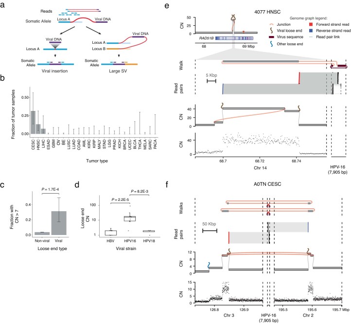
Breakends initiating complex amplifications are themselves likely to be amplified⁴. Viral loose ends were frequently amplified (CN > 7) relative to nonviral loose ends (P = 1.7 × 10⁻⁴; OR = 8.66) (Extended Data Fig. 8c), and HPV-16 loose ends had higher mean CN than either HPV-18 or HBV loose ends (P = 8.2 × 10⁻³ and P = 2.2 × 10⁻⁵, respectively, Extended Data Fig. 8d). Among these was an HNSC tumor (TCGA-4077) locus where two high-copy viral loose ends on chromosome 14 flanking an intronic region of the RAD51B gene were fused to opposite ends of the HPV-16 genome (Extended Data Fig. 8e). This locus is consistent with an ecDNA where HPV-16 is fused between two ends of a long-range duplication junction. This and other similar amplicon structures with high-copy viral loose ends (Extended Data Fig. 8e,f) point to HPV-16 integration as an initiating event in SV evolution, rather than a viral insertion into an existing ecDNA.

Crossover between parental homologs is rare in cancer

We next asked whether loose ends could be used to assess the contribution of aberrant homologous recombination to cancer rearrangements. Homologous recombination-driven crossover between parental homologs (allelic homologous recombination, or AHR) is a hallmark of meiosis³². Although AHR has been observed in somatic cells³³, its contribution to cancer structural variation is unclear. AHR crossovers lead to segmental uniparental disomy (UPD) in approximately half of segregants (Fig. 4a, left). In balanced allelic graphs, AHR crossovers manifest as reciprocal pairs of partially mapped and copy-neutral loose ends on distinct parental homologs (Fig. 4b, left, and Methods). Notably, this form of UPD (AHR-UPD) is mechanistically distinct from UPD arising through progressive acquisition of nonhomologous recombination (for example, end joining)-driven rearrangements and/or chromosomal missegregation (progressive UPD, or P-UPD; Fig. 4a,b, right).

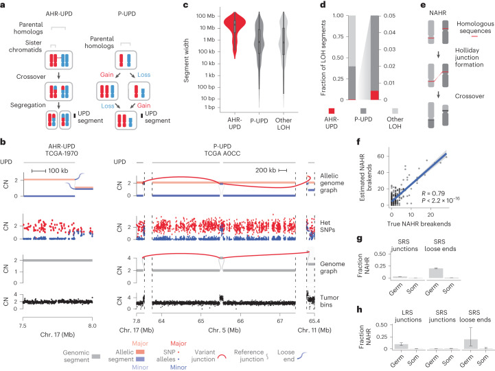
In our simulations (Extended Data Fig. 3a and Methods), JaBbA v1 distinguished AHR-UPD from P-UPD with both high precision (84.4%) and high recall (87.4%), substantially outperforming previous allelic CN algorithms (with precision ranging from 11–44%) (Extended Data Fig. 9a,b). Analysis of segment width distributions showed that AHR-UPD was distinct from P-UPD, whose distribution closely mirrored that of other forms of loss of heterozygosity (LOH; Fig. 4c). Likewise, AHR-UPD events were large (median width of 19.8 Mb), unlike P-UPD events (median width of 0.69 Mb) and other forms of LOH (median width of 0.62 Mb), which were focal (Fig. 4c).

Although AHR was found in many cancers (24% of all tumors) and specific tumor types (for example, 55% of cases of malignant lymphoma) (Extended Data Fig. 9c), it contributed to a minority of UPD events, most of which were progressive (31% P-UPD versus 1% AHR-UPD by total width) (Fig. 4d). Overall, a small minority of detected cancer breakends (<1%) arose by AHR (including non-UPD LOH). On the basis of an approximate rate of 0.5 AHR events per tumor and 100 cell divisions in the average ancestral cancer clone, and barring effects of selection, we estimate a rate of 10⁻¹² AHR events per base pair per cell division. This is four orders of magnitude lower than the rate of meiotic recombination in human gametes, suggesting that AHR events are infrequent in somatic evolution³⁴.

Germline but not somatic loose ends are consistent with NAHR

A second mechanism by which aberrant homologous recombination can cause large SVs is through non-AHR (NAHR), or crossover between long (>500-bp) stretches of nearly identical genomic sequences at distant haploid coordinates^32,35,36 (Fig. 4e). We reasoned that such SVs would engender pairs of loose ends with substantial (>500-bp) strand-specific sequence homology in their vicinity (Extended Data Fig. 10a and Methods)³⁶. Indeed, the burden of homologous loose end pairs accurately reflected the true NAHR burden across a compendium of simulated SRS tumor whole-genome profiles (Extended Data Fig. 3a) harboring a wide range of NAHR SV fractions (1–10%) (Fig. 4f).

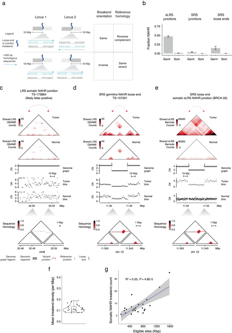
Analyzing breakend pairs within each tumor, we found that approximately 20% of germline loose ends (Methods) were consistent with NAHR in contrast to only about 0.5% of somatic loose ends (and 0.06% of all somatic SV breakends) (Fig. 4g). These findings are consistent with prior observations about the substantial role of NAHR in germline variation^8,37. The somatic NAHR burden did not vary by tumor type nor was it lower in tumors harboring biallelic pathogenic mutations in DNA repair genes, including frequently mutated homologous recombination pathway mediators (BRCA1, BRCA2, PALB2 and RAD51C). In summary, given a mean of 0.16 somatic NAHR events per tumor occurring across an estimated eligible territory of 2.8 × 10⁸ homologous position pairs, we estimate a somatic NAHR density of 6 × 10⁻¹⁰ events per cancer genome bp² (Methods).

To validate these SRS findings in long-molecule whole-genome profiles, we analyzed 38 melanoma and breast cancer cases profiled with SRS and either LRS or sLRS. Both LRS and sLRS data confirmed our SRS findings that somatic NAHR SVs were rare (<1% of LRS junction calls) while germline NAHR SV events were common (Fig. 4h and Extended Data Fig. 10b–e). Notably, we did not identify any reciprocal somatic NAHR rearrangements, a class of SVs that may potentially be missed through analysis of SRS loose ends.

Extrapolating beyond the CN-mappable genome

The analyses described above were limited to the 87% of the genome where CN could be reliably measured with SRS (Fig. 5a). The remaining 13% that is CN-unmappable comprises largely regions in or around telomeres and centromeres (Extended Data Fig. 2b). To assess the burden of large SVs here, we applied two simplifying assumptions: (1) the rate of NAHR between any two regions in the genome is proportional to the number of position pairs with substantial homology (>500 bp with >96% homology) between these regions and (2) the density of non-NAHR-driven rearrangements is uniform across the genome, and hence the burden of non-NAHR breakends in a given region is proportional to its width. Both of these assertions hold true, to a first approximation, across the CN-mappable genome (Extended Data Fig. 10f,g).

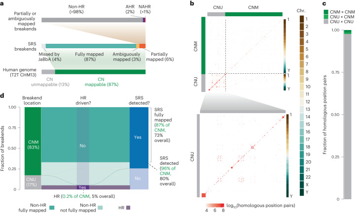
We used the latest telomere-to-telomere build (T2T CHM13; ref. ³⁸) to estimate the number of homologous position pairs outside CN-mappable regions (Fig. 5b). We found that CN-unmappable sequences harbored ~100-fold-greater homologous position pairs (2.7 × 10¹⁰ bp²) than the CN-mappable portion of the T2T CHM13 genome build (2.8 × 10⁸ bp²) (Fig. 5c). This suggested that CN-unmappable regions harbor ~100 times as many NAHR SVs as CN-mappable regions. Integrating these measurements (Fig. 5a–c and Methods), we estimate that CN-mappable regions harbor 83% of all large SV cancer breakends, most of which are detected by SRS (Fig. 5d). Furthermore, even when CN-unmappable regions are taken into account, we estimate that homologous recombination contributes to a small proportion (~5%) of large cancer SV breakends (Fig. 5d).

Discussion

As cancer whole-genome SRS efforts scale and long-molecule genome profiling technologies mature, it is important to understand the limitations of SRS, particularly for the detection of chromosomal alterations. The conventional wisdom in the field has been that SRS misses most SVs owing to the prevalence of repeats in the human genome and the unclear contribution of NAHR to somatic structural genomic evolution^8,37,39,40. Contrary to this prevailing intuition, we find that SRS detects and maps most large (>10-kb) somatic SV breakends in CN-mappable genomic regions. Intuitively, this is because most cancer chromosomal alterations are unbalanced and nonreciprocal (Fig. 1e), thus creating a CN footprint that SRS, when guided by mass balance approaches such as JaBbA v1, can reliably detect (Fig. 1b).

Our SRS analyses suggest that long-molecule technologies (for example, LRS and sLRS) will only modestly improve the detection of chromosomal breakends. We confirm this by jointly profiling the whole genomes of cancer samples and their matched normal samples with deep long-molecule sequencing (LRS or sLRS) and SRS. Given our findings, what additional insight into SVs can long-molecule technologies hope to offer? First, long molecules will enable the phasing of junctions to nearby somatic and germline variants. Resolution of the multi-junction haplotype structure at complex SVs may substantially inform their mechanistic interpretation and functional annotation, as in a recent study from our group¹⁹. Second, long molecules substantially increase the sensitivity for smaller (≤10-kb) somatic SVs, which were excluded from our analyses^41–43. Future long-molecule studies will be needed to uncover the mutational processes and selective pressures driving the evolution of these smaller SV classes, including retrotransposition events.

Our study provides some of the most definitive evidence showing that NAHR drives a small proportion (<1%) of chromosomal alterations, at least in CN-mappable genomic regions. Our NAHR estimates in the remaining 13% (Fig. 5) of the genome assume that CN-mappable and CN-unmappable regions are subject to similar mutational processes. This assertion may require re-evaluation given recent studies investigating centromeric mutational processes⁴⁴. Other settings where homologous recombination has been invoked, such as in the recombination of extrachromosomal DNA (ecDNA)^45,46, may similarly represent unique chromatin environments that are distinct from the remainder of the genome where homologous recombination rarely creates large SVs.

Practically, our study establishes JaBbA v1 as a state-of-the-art algorithm for cancer CN analysis, improving upon JaBbA v0.1 as well as classic ‘change point’-based CN callers (Fig. 1b). The use of mass balance in the JaBbA model provides both superior performance in detecting somatic breakends and a lens into missing cancer SVs. Our study supports the use of JaBbA v1 and, more broadly, SRS in clinical cancer cytogenetics, where whole-genome SRS is poised to become routine in an era of plummeting sequencing costs^47,48.

Methods

Research compliance

The research described below complied with all relevant ethical regulations. Notably, 72 deidentified fresh-frozen samples (36 tumors and 36 matched normal tissues) were collected for SRS and LRS or sLRS profiling and analysis (see below) from patients consented to have their genomes profiled and shared at Memorial Sloan Kettering Cancer Center (MSKCC) under institutional review board approvals MSKCC 00-144, MSKCC 12-245 and MSKCC 16-675. Participants were not compensated.

JaBbA v1 algorithm

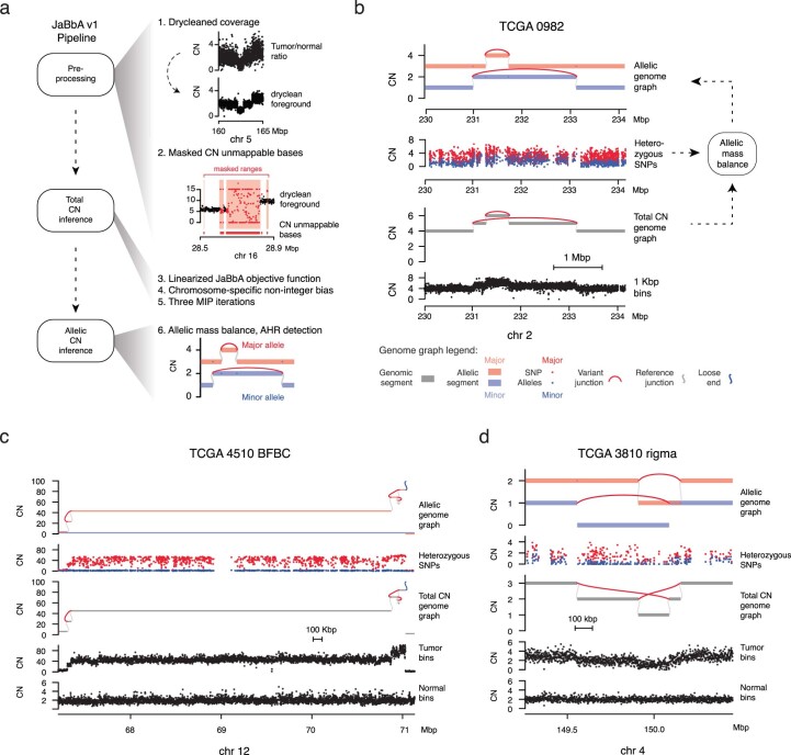
The JaBbA v1 algorithm builds on the previous JaBbA (v0.1) algorithm introduced in Hadi et al.⁴ with two key modifications: (1) updating the JaBbA statistical model to a Laplace distribution, which improved performance and convergence, and (2) balancing allelic genome graphs across parental SNP homologs to enable breakend phasing and identification of allelic loose ends. These and other pipeline changes are visually summarized in Extended Data Figs. 1a and 2a–d. The updated algorithm is described in further detail below.

Genome graph structure

As previously described⁴, JaBbA infers balanced genome graphs through the solution of a mixed-integer program (MIP). A genome graph is a directed graph G = (V, E) whose vertices v₁, v₂ ∈ V represent strands of chromosomal segments and edges e = (v₁, v₂) ∈ E represent segmental adjacencies. Vertices V = V_I ∪ V_N comprise interstitial vertices V_I and ends V_N. The ends V_N = V_T ∪ V_L further comprise reference chromosome ends V_T and loose ends V_L. Edges E = E_R ∪ E_A ∪ E_L comprise reference edges E_R, variant edges E_A and loose end edges E_L, the latter of which connect each interstitial vertex to its incoming (similarly, outgoing) loose end. We use superscript notation to refer to the incoming and outgoing edges of vertices, for example, \({E}_{{\rm{L}}}^{-}(v)={E}_{{\rm{L}}}\cap {E}^{-}(v)\) and \({E}_{{\rm{L}}}^{+}(v)={E}_{{\rm{L}}}\cap {E}^{+}(v)\) to denote the (single) loose end edge that is upstream and downstream of a vertex v, respectively.

Statistical model

Given an initial genome graph, JaBbA assigns a non-negative integer CN \(\kappa :\{V\cup E\}\to {\mathbb{N}}\) to every vertex and edge of G on the basis of (1) the principle of mass balance and (2) the likelihood of purity- and ploidy-transformed read depth data \(x\in {{\mathbb{R}}}^{n}\) across n genomic bins. The principle of mass balance requires the CN of every vertex to be equal to the sum of its incoming edges and the sum of its outgoing edges, engendering the junction balance constraints

as well as a skew symmetry constraint forcing each vertex v and edge e to have the same CN as its reverse complement \(\bar{v}\) and \(\bar{e}\), respectively.

Each vertex v ∈ V_I(G) represents a genomic segment overlapping bins J(v) ⊆ {1, …, n}, whose read depth x_J(v) is modeled as i.i.d. samples from a Laplace distribution with scale parameter b(v, x, J) and mean κ(v). We also apply an exponential prior with decay parameter λ on the count of fitted loose ends (that is, with CN > 0). Under this model, the maximum a posteriori probability estimate of κ minimizes

subject to junction balance and skew symmetry constraints. Here \(\rho (v,x,J)=\frac{1}{| \,J(v)| }{\sum }_{j\in J(v)}{x}_{j}\) and the scale parameter b models read depth noise, which is set to \(b(v,x,J)={\rm{max}}(1,\sqrt{\rho (v,x,J)})\). Finally, we allow the user to specify edges E_F ⊆ E (for example, high-confidence junctions) to force-incorporate into the balanced genome graph. This defines the MIP as follows:

The solution of equation (3) yields a balanced genome graph (G, κ), which minimizes the number of loose ends used (that is, with CN > 0) while maximizing the likelihood of the read depth data x. The use of a Laplace instead of a Gaussian distribution in the likelihood allows the solution of a linear rather than a quadratic MIP, substantially improving scale and convergence relative to the previous formulation⁴. See Supplementary Note 1 for a full derivation.

Allelic mass balance

We extended JaBbA to use mass balance in the inference of allele-specific CN. To do so, we generate an allelic genome graph \(\hat{G}\) from the original (total CN) balanced genome graph (G, κ), where every vertex in G gives rise to two allelic vertices in \(\hat{G}\) and every edge in G gives rise to four allelic edges in \(\hat{G}\). In addition to junction balance (equation (1)) and skew symmetry (equation (3)) constraints, we constrain the CN of allelic vertices mapping to a given vertex v in G to sum to that vertex’s total CN κ(v) (similarly for edges). We additionally allow at most one of the four variant edges in \(\hat{G}\) that arise from the same variant edge in G to have nonzero CN. We also allow at most one of the two incoming (similarly, outgoing) reference edges associated with an allelic node in \(\hat{G}\) to have nonzero CN. The latter two constraints apply the ‘infinite sites’ assumption, which states that each variant could have occurred only once in evolution (and hence on a single parental homolog). To balance the allelic genome graph, we solve a MIP that identifies the allelic vertex and edge CN assignment that maximizes the probability of allelic counts subject to these constraints. Full details of allelic mass balance are provided in Supplementary Note 1.

JaBbA v1 pipeline

In addition to algorithmic improvements, the JaBbA v1 pipeline includes additional data processing improvements compared to the previous version⁴: (1) correction of sample-specific bias in tumor read depth and (2) rigorous definition of CN-mappable regions. Unlike previously⁴, 1-kb binned read depth x is obtained via dryclean⁵³, a robust principal-components analysis-based algorithm to remove systematic low-rank biases in binned read depth using a panel of normal samples (Supplementary Note 2). In addition, we mask bins that occur in CN-unmappable regions of the genome (see below for details) and use purity and ploidy estimates to transform read depth into CN units (Supplementary Note 2). The JaBbA v1 pipeline then applies CBS⁵⁴ to x and takes the union of the resulting segment endpoints with SvAbA²² junction breakends to construct a preliminary genome graph.

In practice, we use three iterations of total CN MIP optimization (equation (3)) followed by allelic mass balance. After each total CN iteration, the results are processed to yield a simplified graph where reference adjacent segments are merged if a loose end or variant junction with CN > 0 does not exist at their interface. The first MIP iteration takes as input only large (>10-kb) and high-confidence (FILTER = PASS) SvAbA junctions and CBS segment breakends. Clusters of high-confidence reciprocal SVs are constrained into the model (that is, by including in the set E_F in equation (3)). The second MIP iteration augments the graph from the first iteration with low-confidence SvAbA junctions located within 10 kb of fitted loose ends. The final MIP iteration refits the graph from the second iteration but adds a noninteger chromosome-specific offset that prevents hypersegmentation from small inaccuracies in purity and ploidy estimation or subclonal CN changes. Allelic mass balance is then run on the balanced genome graph output of the final MIP iteration. To optimize AHR detection, before allelic mass balance, large (>1-Mb) segments of the balanced genome graph are further split by running CBS on minor allelic count vectors (see Supplementary Note 2 for details of chromosomal bias correction and AHR detection).

Mappability analysis

We performed exhaustive self-alignment of all 101-mers in the GRCh37 reference to identify base-unmappable positions, that is, those whose corresponding 101-mer gave rise to at least one full-length supplementary alignment or harbored at least one masked (N) base. A position was then called CN-unmappable if more than 90% of the bases in a 1-kb window around that position were base-unmappable; otherwise, it was called CN-mappable. An analogous approach was used to determine GRCh38 and 150-bp mappability (Extended Data Fig. 2d). Additional details are provided in Supplementary Note 2.

Short-read whole-genome sequencing

SRS whole-genome profiles for 1,330 high-purity (>0.5) tumors (inferred sex: 586 female, 744 male; age: 4–90 years, 164 unknown) and 326 cell lines (provided sex: 139 female, 170 male, 17 unknown; age: 0.25–74.05 years, 46 unknown) were obtained from a previous study published by Hadi et al.⁴. Additional SRS whole-genome libraries were prepared using the Illumina TruSeq DNA PCR-free Library Preparation Kit and profiled on an Illumina NovaSeq 6000 sequencer with 2 × 150-bp cycles. Following GRCh37 alignment, data processing and standard whole-genome variant calling, we ran the JaBbA v1 pipeline (see above) and previously published somatic CN callers (JaBbA v0.1 (ref. ⁴), ASCAT v2.5.2 (ref. ¹⁴), FACETS v0.6.2 (ref. ¹⁷), Sequenza v3.0.0 (ref. ¹⁶) and TITAN v1.28 (ref. ¹⁵)). Additional details regarding SRS library preparation, data processing and variant calling are provided in Supplementary Note 3.

Long-read whole-genome sequencing

LRS profiles were generated for ten melanomas and one triple-negative breast cancer collected at MSKCC (collection details above; inferred sex: six female, five male; age: >17 years). Following high-molecular-weight (HMW) DNA extraction, LRS was performed on the Oxford Nanopore Technologies PromethION sequencer using R10 chemistry with two flow cells per tumor and one flow cell per normal sample. Following GRCh37 long-read alignment (minimap2 v2.17), LRS SV junction calls were identified from the two-way consensus of four callers: cuteSV (release v2.0.2; ref. ⁵⁰), SAVANA (release 0.2.3; ref. ⁵²), SVIM (release 2.0.0; ref. ⁴⁹) and Sniffles2 (release v2.0.7; ref. ⁵¹). Callers were run on tumor and normal samples separately (cuteSV, SVIM, Sniffles2) or in paired mode (SAVANA). Tumor and normal junction calls with identical orientation and 1-kb padded overlap were merged across algorithms. Additional details regarding LRS library preparation and data processing are provided in Supplementary Note 4.

Synthetic long-read whole-genome sequencing

sLRS whole-genome profiling was performed on 25 breast cancer tumor–normal pairs (collection details above; inferred sex: 25 female, 0 male; age: >17 years) and a panel of 8 ATCC cell lines (provided sex: 5 male, 3 female; age: unknown) previously profiled with SRS by the Cancer Cell Line Encyclopedia⁵⁵. In brief, HMW DNA was subjected to 10x Genomics Chromium Genome library preparation and sequenced on an Illumina NovaSeq 6000 sequencing system to approximately 30× base and 170× physical coverage. 10x Genomics linked reads were aligned to GRCh37 using the EMerAld aligner (v0.6.2)⁵⁶. To nominate SV junctions, we applied a consensus of three algorithms (LinkedSV, https://github.com/WGLab/LinkedSV (commit 1b77a14)⁵⁷; GROC-SV, https://github.com/grocsvs/grocsvs (v0.2.6)⁵⁸; NAIBR, https://github.com/raphael-group/NAIBR (commit 15eba96)⁵⁹) run on tumor and normal sLRS alignments. Tumor and normal junction calls with identical orientation and 1-kb padded overlap were merged across algorithms. Somatic SVs were then called as junctions found in tumors by two or more algorithms and undetected in the normal sample. Additional details regarding sLRS profiling and data processing are provided in Supplementary Note 4.

Short- versus long-read platform comparisons

We used 1-kb strand-specific overlap of SRS breakends (junctions and loose ends) and LRS/sLRS junction breakends to assess concordance between SV calling platforms. To assess the ability of LRS or sLRS junctions to resolve SRS loose ends, we applied an additional iteration of junction balance to SRS-derived balanced genome graphs, including additional LRS or sLRS junctions as input. We then overlapped loose ends in the original SRS genome graph with junctions incorporated into the LRS/sLRS genome graph. If a loose end was within 1 kb of an LRS breakend or within 10 kb of an sLRS junction breakend on the same strand, we considered that loose end to have been resolved by LRS/sLRS. We applied gGnome⁴ to annotate and compare complex SV events across SRS, LRS and sLRS JaBbA graphs and used genomic overlaps to identify shared versus platform-specific calls.

Loose end classification

To identify candidate distal mappings for loose ends, we used Fermi⁶⁰ local assembly (https://github.com/mskilab-org/RSeqLib) and realignment of loose end-associated reads and mates. Fermi contigs were assessed for tumor and normal read support through BWA realignment of reads to contigs and the reference (https://github.com/mskilab-org/readsupport) to uncover tumor-specific contigs with distal alignments. To find additional distal mappings, we also analyzed consensus distal alignments of loose end-associated reads. We then labeled loose ends as ‘fully mapped’ or ‘ambiguously mapped’, respectively, if they had a unique or ambiguous tumor-specific distal mapping and ‘partially mapped’ otherwise. See Supplementary Note 5 for full details of loose end classification.

Neotelomere analysis and validation

We identified telomere repeat-positive sequences as those matching one of a panel of G-rich and C-rich telomere repeat trimers and their six cyclic permutations. A loose end was considered telomere repeat-positive if a tumor-specific telomere repeat-positive contig (see above) was found at the loose end. Given an sLRS telomere repeat-positive loose end, we counted read pairs comprising exclusively telomere repeats across all sLRS barcodes associated with the locus and multiplied the maximum value by the median intramolecular distance between reads across all molecules in that sLRS library to estimate the neotelomere length. To validate neotelomere candidates, genomic DNA was isolated from U2OS and Saos-2 cells and, where indicated, treated with Bal-31 exonuclease²⁴. Bal-31-digested DNA was isolated by phenol extraction and ethanol precipitation and was then digested with the appropriate restriction enzyme. Gel electrophoresis of the DNA, Southern blotting and hybridization with Klenow-labeled radioactive probes were performed. See Supplementary Note 5 for additional details of neotelomere analysis and validation.

Nominating NAHR junctions

We identified all pairs of sequences with ≥500 bp of homology (96% sequence identity) through exhaustive BWA-mem self-alignment of all 101-mers on both strands of GRCh37. Loose ends b₁ and b₂ were annotated as a putative NAHR junction if a sequence of ≥500 bp within 10 kb of b₁ on its forward strand was found to be homologous to a sequence within 10 kb of b₂ on its negative strand (Extended Data Fig. 10a). Similarly, junctions were annotated as NAHR if their breakends b₁ and b₂ demonstrated the above property.

Distinguishing mechanisms of UPD

After allelic CN inference using JaBbA or other tools, UPD segments (total CN = 2 and minor allele CN = 0) were identified. UPD segments reference adjacent to another segment of CN = 2 without LOH (minor allele CN = 1) were called AHR-UPD; otherwise, segments were called P-UPD.

Simulating tumor and normal SV profiles

We simulated 500 SRS whole-genome SV profiles on GRCh37 by rearranging the fully phased NA12878 Platinum genome⁶¹. To simulate phased rearrangement junctions, we randomly sampled and shifted pan-cancer SvAbA junctions⁴ and assigned each a random NA12878 haplotype. We also simulated NAHR junctions at a prevalence of 0.1–10% by linking pairs of homologous positions in the genome. Junction breakends were used to define allelic segments, and both were assigned a phased integer CN (‘balance’ function, gGnome⁴) with a target ploidy. We sampled junctions to simulate imperfect sensitivity for junction detection (accounting for sampling effects due to finite read depth or stromal admixture) at a rate proportional to tumor purity. Realistic purity and ploidy values were sampled from pan-cancer distributions⁴. To simulate read depth at bins or SNPs, the normalized purity-adjusted CN of each 1-kb bin was multiplied by a coverage factor to achieve a target genome-wide per-base read depth (80× in tumors and 40× in normal samples) and a bias factor was computed from normalized read counts for that bin in a random normal diploid sample. This product was used as the mean parameter for a Poisson distribution, which was sampled to obtain the final total (or allelic) read depth. See Supplementary Note 6 for additional simulation details.

Benchmarking

To benchmark breakend detection, we compared the endpoints of simulated ‘ground-truth’ breakends to CN calls from JaBbA v1 (this paper), JaBbA v0.1 (ref. ⁴), ASCAT (v2.5.2)¹⁴, FACETS (v0.6.2)¹⁷, Sequenza (v3.0)¹⁶ and TITAN (v1.28)¹⁵. True-positive breakends were defined as those found within 10 kb of a ground-truth breakend on the same strand. We applied a similar approach to assess true-positive rates among JaBbA v1 versus v0.1 loose ends. To assess the accuracy of total CN inference, we computed the root mean square error between estimated and ground-truth total (or allelic) CN values across 10-kb genomic bins. See Supplementary Note 6 for additional benchmarking details.

Identifying NAHR-eligible sites in T2T CHM13 v2

We sampled 1 million 500-bp substrings from T2T CHM13 and realigned them to T2T CHM13 using BWA-mem, identifying all alignments with cigar 500M. This yielded nearly 9 million position pairs (p₁, p₂), where p₁ and p₂ represent the starting coordinate of the query and alignment, respectively. We then divided the self-alignments into three categories (CNU × CNU, CNM × CNU and CNM × CNM) on the basis of the overlap of p₁ and p₂ with a CN-mappable region lifted from GRCh37 to T2T CHM13. See Supplementary Note 7 for details of T2T CHM13 NAHR analysis.

Estimating the genome-wide unmappable breakend fraction

To extrapolate SRS findings from the CN-mappable to the CN-unmappable genome, we applied two principles. First, NAHR rearrangements occur in proportion to the number of homologous position pairs in the genome. Second, non-NAHR rearrangements (including AHR and non-HR SVs including end joining) occur in proportion to the number of bases in the genome. Our CN-mappable NAHR analysis found 216 somatic NAHR events across 2.8 × 10⁸ NAHR-eligible position pairs in 1,330 genomes, giving a somatic NAHR density of 6 × 10⁻¹⁰ events per bp². Given the 2.7 × 10¹⁰ NAHR positions in the 13% of the genome that is CN-unmappable, we estimate an approximate NAHR burden of 16.2 breakends per tumor genome. Given the 681 AHR and 357,000 non-HR CN-mappable breakends in the 1,330 tumor samples, we estimate 0.6 AHR and 310 non-HR events per genome. Putting these numbers together, we estimate that ~17% of large SV breakends occur in CN-unmappable regions, and, given JaBbA’s 96% recall in CN-mappable regions, 80% of large SV breakends will be detected and 73% will be fully resolved by SRS. Given an estimated HR burden of 16.8 SVs per tumor genome, the fractional HR SV burden is approximately 5%. See Supplementary Note 7 for additional details of these calculations.

Statistics and reproducibility

All statistical analysis was performed as stated in the figure legends using the R programming language (v4.0.2). Statistical methods were not used to predetermine sample size. The study design did not involve blinding or randomization. See Supplementary Note 8 for additional details on statistics and reproducibility as well as loose end association analyses.

Reporting summary

Further information on research design is available in the Nature Portfolio Reporting Summary linked to this article.

Online content

Any methods, additional references, Nature Portfolio reporting summaries, source data, extended data, supplementary information, acknowledgements, peer review information; details of author contributions and competing interests; and statements of data and code availability are available at 10.1038/s41588-023-01540-6.

References

1. FJ Sedlazeck, H Lee, CA Darby, MC Schatz. Piercing the dark matter: bioinformatics of long-range sequencing and mapping. Nat. Rev. Genet., 2018. [DOI | PubMed]
2. AJ de Koning, W Gu, TA Castoe, MA Batzer, DD Pollock. Repetitive elements may comprise over two-thirds of the human genome. PLoS Genet., 2011. [DOI | PubMed]
3. Y Li. Patterns of somatic structural variation in human cancer genomes. Nature, 2020. [DOI | PubMed]
4. K Hadi. Distinct classes of complex structural variation uncovered across thousands of cancer genome graphs. Cell, 2020. [DOI | PubMed]
5. 5.Cortés-Ciriano, I., Gulhan, D. C., Lee, J. J.-K., Melloni, G. E. M. & Park, P. J. Computational analysis of cancer genome sequencing data. Nature Rev. Genet.23, 298–314 (2021).
6. L Yang. Diverse mechanisms of somatic structural variations in human cancer genomes. Cell, 2013. [DOI | PubMed]
7. Y Drier. Somatic rearrangements across cancer reveal classes of samples with distinct patterns of DNA breakage and rearrangement-induced hypermutability. Genome Res., 2013. [DOI | PubMed]
8. A Malhotra. Breakpoint profiling of 64 cancer genomes reveals numerous complex rearrangements spawned by homology-independent mechanisms. Genome Res., 2013. [DOI | PubMed]
9. CMB Carvalho, JR Lupski. Mechanisms underlying structural variant formation in genomic disorders. Nat. Rev. Genet., 2016. [DOI | PubMed]
10. P Medvedev, M Fiume, M Dzamba, T Smith, M Brudno. Detecting copy number variation with mated short reads. Genome Res., 2010. [DOI | PubMed]
11. CD Greenman. Estimation of rearrangement phylogeny for cancer genomes. Genome Res., 2012. [DOI | PubMed]
12. AW McPherson. Remixt: clone-specific genomic structure estimation in cancer. Genome Biol., 2017. [DOI | PubMed]
13. S Aganezov, BJ Raphael. Reconstruction of clone- and haplotype-specific cancer genome karyotypes from bulk tumor samples. Genome Res., 2020. [DOI | PubMed]
14. EM Ross, K Haase, P Van Loo, F Markowetz. Allele-specific multi-sample copy number segmentation in ASCAT. Bioinformatics, 2021. [DOI | PubMed]
15. G Ha. TITAN: inference of copy number architectures in clonal cell populations from tumor whole-genome sequence data. Genome Res., 2014. [DOI | PubMed]
16. F Favero. Sequenza: allele-specific copy number and mutation profiles from tumor sequencing data. Ann. Oncol., 2015. [DOI | PubMed]
17. R Shen, VE Seshan. FACETS: allele-specific copy number and clonal heterogeneity analysis tool for high-throughput DNA sequencing. Nucleic Acids Res., 2016. [DOI | PubMed]
18. JA Wala. Svaba: genome-wide detection of structural variants and indels by local assembly. Genome Res., 2018. [DOI | PubMed]
19. J Setton. Long-molecule scars of backup DNA repair in BRCA1- and BRCA2-deficient cancers. Nature, 2023. [DOI | PubMed]
20. FP Barthel. Systematic analysis of telomere length and somatic alterations in 31 cancer types. Nat. Genet., 2017. [DOI | PubMed]
21. L Sieverling. Genomic footprints of activated telomere maintenance mechanisms in cancer. Nat. Commun., 2020. [DOI | PubMed]
22. AOM Wilkie, J Lamb, PC Harris, RD Finney, DR Higgs. A truncated human chromosome 16 associated with α thalassaemia is stabilized by addition of telomeric repeat (TTAGGG)n. Nature, 1990. [DOI | PubMed]
23. GB Morin. Recognition of a chromosome truncation site associated with α-thalassaemia by human telomerase. Nature, 1991. [DOI | PubMed]
24. TD Lange. Structure and variability of human chromosome ends. Mol. Cell. Biol., 1990. [PubMed]
25. J Maciejowski, T de Lange. Telomeres in cancer: tumour suppression and genome instability. Nat. Rev. Mol. Cell Biol., 2017. [DOI | PubMed]
26. CA Lovejoy. Loss of ATRX, genome instability, and an altered DNA damage response are hallmarks of the alternative lengthening of telomeres pathway. PLoS Genet., 2012. [DOI | PubMed]
27. M Zapatka. The landscape of viral associations in human cancers. Nat. Genet., 2020. [DOI | PubMed]
28. DL Cameron. VIRUSBreakend: viral integration recognition using single breakends. Bioinformatics, 2021. [DOI | PubMed]
29. 29.Symer, D. E. et al. Diverse tumorigenic consequences of human papillomavirus integration in primary oropharyngeal cancers. Genome Res.32, 55–70 (2021).
30. K Akagi. Intratumoral heterogeneity and clonal evolution induced by HPV integration. Cancer Discov., 2023. [DOI | PubMed]
31. 31.Li, J. S. Z. et al. Chromosomal fragile site breakage by EBV-encoded EBNA1 at clustered repeats. Nature616, 504–509 (2023).
32. M Sasaki, J Lange, S Keeney. Genome destabilization by homologous recombination in the germ line. Nat. Rev. Mol. Cell Biol., 2010. [DOI | PubMed]
33. KA Choate. Mitotic recombination in patients with ichthyosis causes reversion of dominant mutations in KRT10. Science, 2010. [DOI | PubMed]
34. VG Cheung, JT Burdick, D Hirschmann, M Morley. Polymorphic variation in human meiotic recombination. Am. J. Hum. Genet., 2007. [DOI | PubMed]
35. JM Kidd. Mapping and sequencing of structural variation from eight human genomes. Nature, 2008. [DOI | PubMed]
36. J Renkawitz, CA Lademann, S Jentsch. Mechanisms and principles of homology search during recombination. Nat. Rev. Mol. Cell Biol., 2014. [DOI | PubMed]
37. DJ Turner. Germline rates of de novo meiotic deletions and duplications causing several genomic disorders. Nat. Genet., 2021. [DOI]
38. S Nurk. The complete sequence of a human genome. Science, 2022. [DOI | PubMed]
39. MM Parks, CE Lawrence, BJ Raphael. Detecting non-allelic homologous recombination from high-throughput sequencing data. Genome Biol., 2015. [DOI | PubMed]
40. 40.Pascarella, G. et al. Recombination of repeat elements generates somatic complexity in human genomes. Cell185, 3025–3040 (2022).
41. S Aganezov. Comprehensive analysis of structural variants in breast cancer genomes using single-molecule sequencing. Genome Res., 2020. [DOI | PubMed]
42. M Nattestad. Complex rearrangements and oncogene amplifications revealed by long-read DNA and RNA sequencing of a breast cancer cell line. Genome Res., 2018. [DOI | PubMed]
43. FJ Sedlazeck. Accurate detection of complex structural variations using single-molecule sequencing. Nat. Methods, 2018. [DOI | PubMed]
44. 44.Saayman, X., Graham, E., Nathan, W. J., Nussenzweig, A. & Esashi, F. Centromeres as universal hotspots of DNA breakage, driving RAD51-mediated recombination during quiescence. Mol. Cell83, 523–538 (2023).
45. RT Schimke. Gene amplification in cultured animal cells. Cell, 1984. [DOI | PubMed]
46. C Rosswog. Chromothripsis followed by circular recombination drives oncogene amplification in human cancer. Nat. Genet., 2021. [DOI | PubMed]
47. EJ Duncavage. Genome sequencing as an alternative to cytogenetic analysis in myeloid cancers. N. Engl. J. Med., 2021. [DOI | PubMed]
48. 48.Almogy, G. et al. Cost-efficient whole genome-sequencing using novel mostly natural sequencing-by-synthesis chemistry and open fluidics platform. Preprint at bioRxiv10.1101/2022.05.29.493900 (2022).
49. D Heller, M Vingron. SVIM: structural variant identification using mapped long reads. Bioinformatics, 2019. [DOI]
50. T Jiang. Long-read-based human genomic structural variation detection with cuteSV. Genome Biol., 2020. [DOI | PubMed]
51. 51.Smolka, M. et al. Comprehensive structural variant detection: from mosaic to population-level. Preprint at bioRxiv10.1101/2022.04.04.487055 (2022).
52. H Elrick. Abstract LB080: SAVANA: a computational method to characterize structural variation in human cancer genomes using nanopore sequencing. Cancer Res., 2023. [DOI]
53. 53.Deshpande, A., Walradt, T., Hu, Y., Koren, A. & Imielinski, M. Robust foreground detection in somatic copy number data. Preprint at bioRxiv10.1101/847681 (2019).
54. 54.Olshen, A. B., Venkatraman, E. S., Lucito, R. & Wigler, M. Circular binary segmentation for the analysis of array-based DNA copy number data. Biostatistics10.1093/biostatistics/kxh008 (2004).
55. M Ghandi. Next-generation characterization of the Cancer Cell Line Encyclopedia. Nature, 2019. [DOI | PubMed]
56. A Shajii, I Numanagić, B Berger. Latent variable model for aligning barcoded short-reads improves downstream analyses. Res. Comput. Mol. Biol., 2018. [PubMed]
57. L Fang. Linkedsv for detection of mosaic structural variants from linked-read exome and genome sequencing data. Nat. Commun., 2019. [DOI | PubMed]
58. N Spies. Genome-wide reconstruction of complex structural variants using read clouds. Nat. Methods, 2017. [DOI | PubMed]
59. R Elyanow, H-T Wu, BJ Raphael. Identifying structural variants using linked-read sequencing data. Bioinformatics, 2018. [DOI | PubMed]
60. H Li. Exploring single-sample SNP and indel calling with whole-genome de novo assembly. Bioinformatics, 2012. [DOI | PubMed]
61. MA Eberle. A reference data set of 5.4 million phased human variants validated by genetic inheritance from sequencing a three-generation 17-member pedigree. Genome Res., 2017. [DOI | PubMed]
62. JJ-K Lee. Tracing oncogene rearrangements in the mutational history of lung adenocarcinoma. Cell, 2019. [DOI | PubMed]
63. TG Paulson. Somatic whole genome dynamics of precancer in Barrett’s esophagus reveals features associated with disease progression. Nat. Commun., 2022. [DOI | PubMed]
64. S Baca. Punctuated evolution of prostate cancer genomes. Cell, 2013. [DOI | PubMed]