Heterogeneous data integration methods for patient similarity networks
Abstract
Patient similarity networks (PSNs), where patients are represented as nodes and their similarities as weighted edges, are being increasingly used in clinical research. These networks provide an insightful summary of the relationships among patients and can be exploited by inductive or transductive learning algorithms for the prediction of patient outcome, phenotype and disease risk. PSNs can also be easily visualized, thus offering a natural way to inspect complex heterogeneous patient data and providing some level of explainability of the predictions obtained by machine learning algorithms. The advent of high-throughput technologies, enabling us to acquire high-dimensional views of the same patients (e.g. omics data, laboratory data, imaging data), calls for the development of data fusion techniques for PSNs in order to leverage this rich heterogeneous information. In this article, we review existing methods for integrating multiple biomedical data views to construct PSNs, together with the different patient similarity measures that have been proposed. We also review methods that have appeared in the machine learning literature but have not yet been applied to PSNs, thus providing a resource to navigate the vast machine learning literature existing on this topic. In particular, we focus on methods that could be used to integrate very heterogeneous datasets, including multi-omics data as well as data derived from clinical information and medical imaging.
Article type: Review Article
Keywords: patient similarity networks, biomedical applications, multimodal data, data fusion
Affiliations: AnacletoLab – Computer Science Department, Universitá degli Studi di Milano, Via Celoria 18, 20135, Milan, Italy; European Commission, Joint Research Centre (JRC), Ispra (VA), Italy; CINI, Infolife National Laboratory, Roma, Italy; Department of Computer Science, Royal Holloway, University of London, Egham, TW20 0EX UK; School of Applied Mathematics (EMAp), Fundação Getúlio Vargas, Rio de Janeiro Brazil; DSRC UNIMI, Data Science Research Center, Milano, 20135, Italy; ELLIS, European Laboratory for Learning and Intelligent Systems, Berlin, Germany
License: © The Author(s) 2022. Published by Oxford University Press. CC BY 4.0 This is an Open Access article distributed under the terms of the Creative Commons Attribution License (https://creativecommons.org/licenses/by/4.0/), which permits unrestricted reuse, distribution, and reproduction in any medium, provided the original work is properly cited.
Article links: DOI: 10.1093/bib/bbac207 | PubMed: 35679533 | PMC: PMC9294435
Relevance: Moderate: mentioned 3+ times in text
Full text: PDF (1.8 MB)
Introduction
In the last decades, medical research has begun to move from a population-based perspective to a personalized one, often referred to as precision medicine, where patients’ biomedical characteristics are leveraged for diagnosis, prognosis and choice of appropriate treatment [ref. 1, ref. 2]. In this context, it is widely accepted that if two patients share similar clinical variables and omics profiles, their clinical outcomes should also be similar. Pairwise similarities between patients have a natural representation as graphs—Patient Similarity Networks (PSN)—where nodes represent patients and edges represent the similarity between patients calculated using their clinical and/or biomolecular features. In this framework unsupervised clustering methods and supervised classification models that leverage similarities between patients have been successfully applied to stratify patients and to predict their phenotype or clinical outcome [ref. 3–8]. Representing data as graphs provides several advantages, including interpretability and privacy [ref. 9], as patient-specific information cannot be recovered from the similarity measures.
The increasing availability of high-throughput technologies able to generate high-dimensional, distributed biomedical datasets, ranging from multi-omics [ref. 8] to imaging [ref. 10], clinical and demographic data [ref. 11], calls for approaches to mine and aggregate salient information [ref. 12] with the ultimate aim of building PSNs integrating such diverse datasets. However, the majority of PSNs that have been proposed are built using only one source of information. At the same time, several methods that can integrate heterogenous sources of information into graph structures have appeared in the past decades in the biomedical and machine learning literature.
In this article, we review existing methods for integrating multiple biomedical data views to construct PSNs. Since the type of data being integrated and the specific integration method must be coupled with an appropriate choice of similarity measure, we will also discuss different similarity measures. Importantly, this paper also reviews methods for integrating information into graph structures that appeared in the machine learning literature but have not yet been used for PSNs. We believe that this will be beneficial for the reader, providing a resource to navigate the vast machine learning literature existing on this topic, and possibly inspire the use and development of novel techniques of data integration for PSNs. Moreover, unlike earlier reviews (see e.g. [ref. 8, ref. 13–16]), we focus on methods that may be used for patients’ classification and clustering that integrate not only multi-omics data, but also clinical and image sources.
We propose a taxonomy that groups existing methods for building PSNs into three main categories. ’PSN-fusion methods’ [ref. 3, ref. 6, ref. 17] build different PSNs, one for each data source, that are then fused together into a single PSN. ’Input data-fusion’ methods [ref. 18–21] combine the different data sources into a single dataset that is then used for building a single PSN. Finally, ’Output-fusion methods’ [ref. 22–24] build different PSNs, one for each data source, that are analyzed separately, and results are then combined.
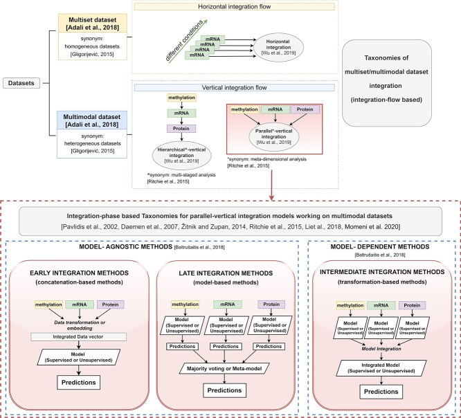
Other multimodal data-fusion surveys not specific for PSNs have been proposed in the bioinformatics field by adopting different taxonomies (schematized in Figure 1, Appendix A). Some taxonomies focus on the type of multi-datasets being integrated, thus identifying ’horizontal integration techniques’ [ref. 25] (top of Figure 1-yellow box) and ’vertical integration techniques’ [ref. 25] (top of Figure 1-light blue box). While the former fuse ’homogeneous multisets’ [ref. 26], i.e. ’multimodal datasets’ where each view produces the same data type under different settings, the latter integrate the classic ’heterogeneous’ [ref. 26] multimodal datasets. Vertical integration techniques are further classified into methods applying a ’hierarchical (alias ’multi-staged’ [ref. 27]) integration’ flow, where ground knowledge about the relationships between the different views is considered during the integration, and methods applying a ’parallel (alias ’meta-dimensional’ [ref. 27]) integration’ flow (bottom of Figure 1-red-dashed box), where each view is processed in a similar but independent way. Parallel integration methods are the most diffused in literature given their generalizability. For this reason several reviews concentrate solely on them and introduce taxonomies that distinguish, e.g. ’model-agnostic’ versus ’model-dependent’ methods [ref. 28], or exploit an ’early–intermediate–late’ taxonomy [ref. 27, ref. 29–33] (described in detail in Appendix A).
Each review paper focuses on different aspects of the multimodal data integration. For example, some works solely focus on integrative unsupervised clustering techniques [ref. 34] or supervised multi-omics prediction models [ref. 29, ref. 33, ref. 35], or survey data-fusion techniques that are either applied to multi-omics data [ref. 16, ref. 25–27, ref. 36], or that apply specific data-fusion techniques (e.g. integrative Bayesian models [ref. 13, ref. 37] or multimodal neural networks [ref. 38]).
Unlike previous reviews, this work specifically focuses on integrative methods for PSN-based models integrating not only multi-omics data, but also clinical and imaging sources. Each method is critically described to highlight its main advantages and drawbacks, enabling the reader to select the most appropriate approach to answer her/his scientific questions.
Given a set of patients and their corresponding clinical and biomolecular features, the topology of the corresponding PSN depends crucially on how the similarity measure is calculated. Therefore, we begin describing the similarity measurement methods presented in the literature. Our taxonomy of existing methods for building PSNs is described in Sections PSN-fusion methods and Input data-fusion and output-fusion methods. Tables 3–8 summarize the most relevant methods we surveyed.
PSN construction
The construction of the PSN is a crucial step in PSN analysis models, whose effectiveness mainly depends on the available multimodal datasets from which samples are extracted and on the choice of the measure exploited for pairwise similarity computation between samples.
Several kinds of similarity measures have been adopted in literature for PSN construction: classic distance metrics tailored to the data type [ref. 39, ref. 40]; kernel functions [ref. 41, ref. 42] that substitute distance metrics; ‘kernels on graphs’ methods [ref. 43]. In the remainder, we discuss their characteristics.
The usage of classic ’(opportunely inverted) distances’ or ’similarity metrics’ [ref. 39, ref. 40] is often preferred when the data types are normalized and homogeneous. As an example, PSNs on continuous, normalized, data have been constructed by using the cosine similarity [ref. 5, ref. 44], or the Euclidean [ref. 45] or Mahalanobis distance [ref. 45]; PSNs on discrete data types have been built by exploiting the Chi-squared distance [ref. 3, ref. 6]; binary data have been handled by using the Jaccard distance [ref. 46] or many other distance measures (see [ref. 47] for a list of 76 metrics and measures specifically designed for binary data).
When data-blocks with heterogeneous and/or normalized variable types are available, more articulated schemas [ref. 6, ref. 48] have been proposed to integrate different similarity metrics into a unique measure. As an example, in [ref. 48] the authors proposed a supervised Cox regression model to initially learn a weight for each variable; the learnt weights are then used to compute a similarity score as a weighted sum of individual similarities obtained on each feature by using standard metrics. In this way, different similarity metrics can be used on the different variables based on their type, and the influence of each variable to the global similarity score is weighted on the prediction (e.g. survival time when using a Cox regression model). On the other hand, when dealing with datasets composed by continuous non-normalized variable types, Pai et al. [ref. 6] propose computing the average of all the normalized similarities over each variable, where the normalization is essentially a min–max normalization.
When dealing with complex problems, literature works often rely on ’Kernel functions’ [ref. 49] for PSN computation. The rationale behind this choice is based on the assumption that point separability is often improved after a nonlinear projection of points into a higher-dimensional space. Kernel functions are particularly appealing in this context since they express pairwise distances in a higher-dimensional space by directly using the (lower-dimensional) input samples, therefore avoiding the expensive explicit computation of a nonlinear higher-dimensional mapping followed by pairwise similarity evaluation (using the well-known ’kernel-trick’). Even in this case the choice of the kernel function must be tailored to the data type that is crucial to obtain reliable results. In this context, PSNs are often computed in literature methods working on biomedical data by using classic parametric ’normalized linear kernels’ [ref. 30, ref. 50], ’polynomial kernels’ or ’Gaussian kernels’ [ref. 51, ref. 52], whose parameters are tuned to optimize performance. As an example, the prognostic approach presented in [ref. 30] obtains a set of unimodal PSNs by applying normalized linear kernels on each of the data sources containing clinical and multi-omics datasets. In this case, the usage of the same kernel function on different sources is appropriate because they are characterized by the same data type (real-valued data type).
In a subsequent work [ref. 53], the same authors extend the dataset by including categorical and integer data types; therefore, they substitute the linear kernels with a set of kernels tailored on each data type being processed. Of note, the kernels used in [ref. 30, ref. 53] are always normalized. This is a crucial characteristic when integrating multiple kernels because comparable kernel scales are obtained, therefore facilitating the kernel integration. Moreover, in the case of kernel-aggregation systems exploiting weighted averages of the unimodal kernels, normalization also improves the interpretability of the computed integration weights, the latest being directly related to the importance of their respective kernel [ref. 53].
A recent advance in the field of PSN analysis is provided by unsupervised methods that compute the PSN through the ’scaled exponential Euclidean kernel’ [ref. 3] and its modifications [ref. 54, ref. 55]. They essentially apply a local normalization of the distance between a central node and any of its neighbors, so that distances are independent from the neighborhood scales. Their application in the context of unsupervised patient clustering through PSN analysis has obtained promising results [ref. 3] (see Section SNF-based methods).
Given its effectiveness, the scaled Euclidean distance has been extended in [ref. 54] to deal with heterogeneous data types containing continuous and boolean variables. More precisely, the similarity on boolean data is measured by using the weighted Hamming distance with weights computed by supervised approaches or pre-set based on existing knowledge. Further, in [ref. 55] the authors propose adopting the Chebyshev distance instead of the Euclidean distance.
Gliozzo et al. [ref. 7] extend to PSNs a previous ’kernel-based’ approach originally applied to the semi-supervised analysis of biomolecular networks [ref. 56]. More precisely, the authors obtain promising outcome predictions on unimodal PSNs by firstly using the filtered Pearson correlation (by setting to zero all negative values) to measure similarities between unimodal gene expression profiles, and then applying a random walk kernel to strengthen high similarities while diminishing low ones. The neighborhoods identified in the obtained PSN are then used to compute a score for each patient, which is thresholded to obtain the desired classification. While unimodal PSNs are exploited in [ref. 7], the works proposed in [ref. 57] and [ref. 58] exploit random-walks to compute similarities in a multimodal setting.
To improve informativeness, Tables 1 and 2 sketch the similarity measures/ methods used for PSN construction by notable literature works exploiting multimodal datasets; for each paper we report the data types of the different data sources exploited for the investigation, and the similarity measures/methods used for building the corresponding unimodal PSNs.
Table 1: Similarity measures/methods used in literature to build PSNs. For notable works in literature the table reports: the reference of the literature work presenting a multimodal PSN analysis method (column ’References’), the data types (column ’Data type’) of the different sources (column ’Data’) used for the investigation, and the similarity measures/methods exploited for building the unimodal PSNs
| References | Data type | Data | Similarity measure/method |
|---|---|---|---|
| [ref. 46] | Binary | ICD-9 diagnosis code | Jaccard similarity |
| [ref. 44] | Continuous, | Clinical data | Cosine similarity |
| Categorical, discrete | |||
| [ref. 5] | Continuous | Clinical data | Cosine similarity |
| Categorical, discrete | |||
| [ref. 61] | Continuous | mRNA, PPI | Pearson correlation |
| [ref. 7] | Continuous | mRNA | Pearson correlation |
| [ref. 6] | Continuous | Clinical variables | Mean of normalized difference |
| Individual gene | Normalized difference | ||
| Genes in pathways/networks | Pearson correlation | ||
| Discrete | Categorical-ordinal variable | Normalized difference | |
| (e.g. tumor stage) | |||
| Unbinned counts | Shared incidence | ||
| (e.g. mutation data) | in a grouped unit | ||
| Matrix scores | chi-square distance | ||
| (e.g. response to questionnaire) | |||
| [ref. 3] | Continuous | mRNA, miRNA, DNA methylation | Scaled exponential kernel of Euclidean distance |
| Discrete | chi-squared distance | ||
| Binary | agreement-based measure | ||
| [ref. 54] | Continuous binary | mRNA, DNA methylation somatic mutation | Scaled exponential kernel of weighted Euclidean distance scaled exponential kernel of weighted Hamming distance |
| [ref. 62] | Continuous | mRNA, miRNA, DNA methylation | Scaled exponential kernel of Euclidean distance |
| [ref. 63] | Categorical, discrete | Demographic, APOE4 allele status, | squared-exponential kernel |
| MRI | |||
| [ref. 55] | Continuous | Gene expression, | Kernel of Chebyshev distance |
| miRNA, | |||
| Isoform expression | |||
| [ref. 48] | Continuous, categorical, discrete | Clinical data | Weighted sum of distances |
| with weight determined by a scaled | |||
| Cox regression coefficient |
ICD-9: International Classification of Diseases Version 9; CNV: copy number variation; miRNA: micro RNA; MRI: magnetic resonance imaging; mRNA: messenger RNA; PPI: protein–protein interaction
Table 2: Similarity measures/methods used in literature to build PSNs. For notable works in literature the table reports: the reference of the literature work presenting a multimodal PSN analysis method (column ’References’), the data types (column ’Data type’) of the different sources (column ’Data’) exploiting for the investigation, and the similarity measures/methods exploited for building the unimodal PSNs.
| Reference | Data type | Data | Similarity measure/method |
|---|---|---|---|
| [ref. 30, ref. 53] | continuous | mRNA, clinical | normalized linear kernel |
| categorical, discrete, binary | clinical | ||
| [ref. 64] | discrete | MRI | gaussian kernel |
| continuous | CSF | ||
| [ref. 51] | continuous | mRNA, miRNA, CNV, | gaussian kernel |
| DNA methylation, | |||
| discrete | clinical | ||
| [ref. 50] | continuous, | mRNA, miRNA, CNV, | linear kernel |
| DNA methylation, RPPA, | |||
| binary, discrete | somatic mutations, clinical data | ||
| [ref. 65] | continuous | mRNA, CNV, DNA methylation | normalized linear kernel, |
| normalized polynomial kernel, | |||
| normalized gaussian kernel | |||
| [ref. 53] | continuous, categorical (ordinal) | clinical variables | absolute difference of values/ranks of two subjects compared and rescaled using variable range |
| categorical (nominal) | clinical variables | kernel defined using Kronecker delta function | |
| [ref. 57] | continuous, binary | mRNA, RPPA, somatic mutation | novel graph kernel called SmSPK |
CNV: Copy Number Variation; miRNA: micro RNA; mRNA: messenger RNA; RPPA: Reverse-Phase Protein Arrays; CSF: CerebroSpinal Fluid.
Even if a wide range of similarity computation methods has been proposed in literature, a consensus on which strategy performs better on specific data types and problems in the context of precision medicine is still lacking. Some tentative experiments have been conducted for determining the best-performing strategies (see e.g. [ref. 59, ref. 60]), but the lack of common benchmark datasets prevents an unbiased comparison of the different proposed approaches.
PSN-fusion methods
PSN-fusion methods have been specifically developed to process a set of unimodal PSNs and produce an integrated PSN. In Figure 2 we sketch the generic workflow of the PSN-fusion methods. They start by building unimodal PSNs on each data source or data type (Figure 2A). Mind that the choice of the similarity measure/kernel function used to build each PSN (Section PSN construction) is crucial for obtaining informative unimodal PSNs, which would otherwise hamper the achievement of successful results. Next, the aggregation of the unimodal PSNs (Figure 2B) is performed by either Multiple Kernel Learning methods (MKL, Section MKL-based methods, Table 3), which run optimization algorithms inherited from the machine learning field to find the optimal weights of an additive unimodal kernel aggregation, or approaches stemming from the seminal Similarity Network Fusion algorithm (SNF—[ref. 3], Section SNF-based methods, Table 4), which use different strategies to diffuse the similarity information both between neighboring nodes in each unimodal PSN and between corresponding nodes in different PSNs, or other network-based approaches (Section Other PSN-fusion methods and Table 5).
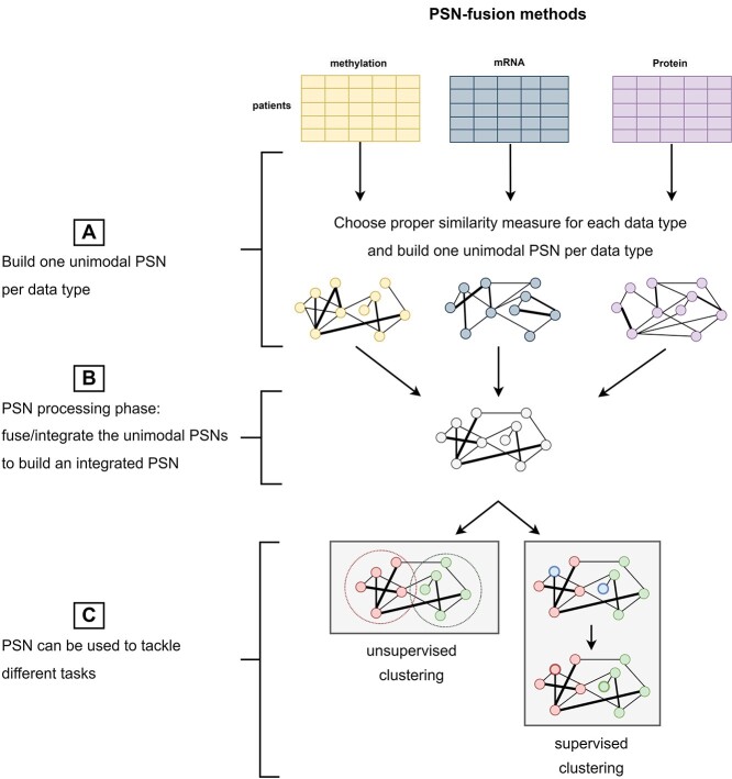
Table 3: MKL-based PSN-fusion methods. For each method, the table reports: the name/acronym with the corresponding reference paper; whether it requires the same set of patients across all data modalities (i.e. ‘Matched Samples’); the dataset used to develop and evaluate the approach in the reference paper and the corresponding sample cardinality and data types composing the dataset; the exploited integration method; the application task and the code availability (with link to the repository and programming languages for which the code is available)
| Name | Matched samples | Dataset | Sample cardinality | Data type | Integration approach | Task | Code and Language |
|---|---|---|---|---|---|---|---|
| PAMOGK\(}{}$^{1}\) | x | TCGA KIRC | 361 | Somatic mutation | MKKM | Unsupervised Clustering | MATLAB, |
| [ref. 57] | NCI-PID at NDEXBio | mRNA | [ref. 77] | (Patient subtype identification) | Python code | ||
| RPPA | |||||||
| [ref. 64] | x | ADNI | 120 | CSF features | MKL | Supervised Classification | |
| MRI | [ref. 17] | (HC versus MCI patients) | |||||
| [ref. 69] | x | TCGA | 585 | Histopathological images | simpleMKL | Supervised Classification | |
| Clinical data | [ref. 17] | (Patient’s Prognosis) | |||||
| mRNA | |||||||
| methy | |||||||
| RPPA | |||||||
| [ref. 67] | x | TCGA GBM | 125 | Histopathological images | simpleMKL | Supervised Classification | |
| CNV | [ref. 17] | (Patient’s Prognosis) | |||||
| mRNA | |||||||
| miRNA | |||||||
| MK-FDA [ref. 73] | x | Protein dataset | Not provided | Protein sequences | MKL | Supervised Multiclass Classification | |
| [ref. 75] | (Protein subcellular localization) | ||||||
| [ref. 50] | x | 14 TCGA datasets | 3382 | Germline variants | MKL | Supervised Classification | |
| Somatic mutation | (Patient’s Survival) | ||||||
| CNV | |||||||
| mRNA | |||||||
| miRNA | |||||||
| methy | |||||||
| [ref. 52] | x | TCGA from | 989 | mRNA | MKL | Unsupervised Clustering | |
| mixOmics | miRNA | (Patients’ subtype identification) | |||||
| methy | |||||||
| rMKL-LPP | x | TCGA GBM | 213 | mRNA | MKL | Unsupervised Clustering | |
| [ref. 76] | TCGA BIC | 105 | miRNA | (Patient subtype identification) | |||
| TCGA KIRC | 122 | methy | |||||
| TCGA LUSC | 106 | ||||||
| TCGA COAD | 92 |
ADNI: Alzheimer’s Disease Neuroimaging Initiative; CNV: Copy Number Variation; CSF: CerebroSpinal Fluid; HC: Healthy Control; MCI: Mild Cognitive Impairment; methy: DNA methylation; miRNA: micro RNA; MKKM: Multiple kernel k-means clustering; MKL: Multiple Kernel Learning; MRI: Magnetic Resonance Imaging; mRNA: messenger RNA; NCI-PID: National Cancer Institute—Pathway Interaction Database; RPPA: Reverse-Phase Protein Arrays; TCGA+cancer code: The Cancer Genome Atlas+ link to complete cancer codes.
Table 4: SNF-based PSN-fusion methods. For each method, the table reports: the name/acronym with the corresponding reference paper; whether it requires the same set of patients across all data modalities (i.e. ‘Matched Samples’); the dataset used to develop and evaluate the approach in the reference paper and the corresponding sample cardinality and data types composing the dataset; the exploited integration method; the application task and the code availability (with link to the repository and programming languages for which the code is available)
| Name | Matched samples | Dataset | Sample cardinality | Data type | Integration approach | Task | Code and Language |
|---|---|---|---|---|---|---|---|
| SNF [ref. 3] | x | TCGA GBM | 215 | mRNA | SNF | Unsupervised Clustering | MATLAB code, R code |
| miRNA | (Patient subtype identification) | ||||||
| methy | |||||||
| ANF [ref. 87] | x | TCGA LUSC | 2193 | mRNA | SNF | Unsupervised Clustering | R code |
| TCGA Adrenal | miRNA | (Patient subtype identification) | |||||
| TCGA Gland | methy | ||||||
| TCGA KIRC | |||||||
| TCGA Uterus | |||||||
| HSNF [ref. 89] | x | TCGA BIC | 105 | mRNA | SNF | Unsupervised Clustering | |
| TCGA GBM | 215 | miRNA | (Patient subtype identification) | ||||
| TCGA KIRC | 122 | methy | |||||
| TCGA LUSC | 106 | ||||||
| TCGA COAD | 92 | ||||||
| SKF [ref. 90] | x | TCGA BIC | 1071 | mRNA | SNF | Unsupervised Clustering | MATLAB code |
| TCGA COAD | 426 | miRNA | (Patient subtype identification) | ||||
| TCGA KIRC | 868 | isoform level | |||||
| TCGA LUSC | 981 | ||||||
| TCGA Stomach | 377 | ||||||
| ab-SNF [ref. 54] | x | TCGA LIHC | Not provided | somatic mutation | SNF | Unsupervised Clustering | R code |
| TCGA KIRP | mRNA | (Patient subtype identification) | |||||
| TCGA BIC | methy | ||||||
| NEMO [ref. 93, ref. 94] | TCGA AML | 3168 across | mRNA | SNF | Unsupervised Clustering | R code | |
| TCGA BIC | all datasets | miRNA | (Patient subtype identification) | ||||
| TCGA COAD | methy | ||||||
| TCGA GBM | |||||||
| TCGA KIRC | |||||||
| TCGA LIHC | |||||||
| TCGA LUSC | |||||||
| TCGA SKCM | |||||||
| TCGA OV | |||||||
| TCGA SARC |
methy: DNA methylation; miRNA: micro RNA; mRNA: messenger RNA; SNF: Similarity Network Fusion; TCGA+cancer code: The Cancer Genome Atlas+ link to complete cancer codes.
Table 5: Other PSN-fusion methods. For each method, the table reports: the name/acronym with the corresponding reference paper; whether it requires the same set of patients across all data modalities (i.e. ‘Matched Samples’); the dataset used to develop and evaluate the approach in the reference paper and the corresponding sample cardinality and data types composing the dataset; the exploited integration method; the application task and the code availability (with link to the repository and programming languages for which the code is available)
| Name | Matched samples | Dataset | Sample cardinality | Data type | Integration approach | Task | Code and Language |
|---|---|---|---|---|---|---|---|
| netDx [ref. 6] | x | TCGA KIRC | 150 | mRNA | Average score | Supervised classification | R code |
| TCGA OV | 252 | miRNA | (patient’s survival) | ||||
| TCGA GBM | 155 | methy | |||||
| TCGA LUSC | 77 | CNV | |||||
| RPPA | |||||||
| clinical data | |||||||
| RWRF, RWRNF [ref. 58] | x | TCGA ACC | 76 | mRNA | RWR | Unsupervised clustering | R code |
| TCGA BLCA | 396 | miRNA | (patient subtype identification) | ||||
| TCGA HNSC | 469 | methy | |||||
| TCGA UVM | 80 | ||||||
| TCGA PAAD | 175 | ||||||
| TCGA THCA | 492 | ||||||
| MRF-MSC [ref. 95] | x | TCGA COAD | 92 | mRNA | Maximization | Unsupervised clustering | |
| TCGA GBM | 215 | miRNA | of alignment to all | (patient subtype identification) | |||
| TCGA BRCA | 105 | methy | the unimodal PSNs | ||||
| TCGA KIRC | 122 | ||||||
| TCGA LSCC | 106 |
CNV: Copy Number Variation; methy: DNA methylation; miRNA: micro RNA; mRNA: messenger RNA; PSN: Patient Similarity Network; RPPA: Reverse Phase Protein Array; RWR: Random Walk Kernel with Restart; TCGA+cancer code: The Cancer Genome Atlas+ link to complete cancer codes.
The integrated PSN may be finally used as input to unsupervised clustering methods aiming at, e.g. identifying patients’ subtypes, or supervised classification methods predicting, e.g. patients’ risk, prognosis or outcome (Figure 2C).
MKL-based methods
Inheriting theories and algorithms from the machine learning fields, MKL methods [ref. 17, ref. 64–66] view the unimodal PSNs as kernels and propose their optimal additive combination, as a weighted sum of the available unimodal kernels. In this context, ‘optimality’ refers to either a ’supervised’ setting or an ’unsupervised’ one.
’Supervised MKL’ algorithms (e.g. simpleMKL [ref. 17]) exploit a supervised classifier model designed to work on the fused kernel. Supervision is guaranteed by the availability of a training set composed of samples whose labels are known. Such training set is used by the chosen supervised MKL method to solve a constrained optimization problem that finds the kernel weights and classifier hyper-parameters maximizing the classification accuracy on the training set. On the other side, ’unsupervised MKL’ methods make no use of labeled samples, but instead solve an optimization problem to find the weights that essentially lead to the maximum alignment between the integrated kernel and any of the input unimodal kernels.
Recent PSN-fusion methods exploiting a ’supervised MKL’ strategy are those presented by [ref. 30, ref. 50, ref. 53, ref. 64, ref. 67]. The work proposed in [ref. 50] designs specific kernels for each omic type in the The Cancer Genome Atlas (TCGA) cancer dataset and then computes the kernel weights by using the training set to optimize the fit of a Cox-survival model.
All the other works [ref. 30, ref. 53, ref. 64, ref. 67] share the use of the kernelized Support Vector Machine (SVM) classifiers [ref. 68], opportunely modified as defined in [ref. 17] and [ref. 66] to work on the kernel resulting from an optimal additive sum. In particular, the works proposed by Daemen et al. [ref. 30, ref. 53] aggregate specific kernels on each clinical data type and uses a classic SVM optimization strategy to derive the optimal weights, while the works proposed in [ref. 64] and [ref. 67] use the easyMKL algorithm to optimize an svm aggregating multiple kernels defined over multimodal datasets also including opportunely coded imaging sources. More precisely, in [ref. 64] authors use the same Gaussian kernels to process both the real cerebrospinal fluid (CSF) biomarkers features and the shape and texture features extracted to code magnetic resonance images (MRI). On the other side, the work proposed in [ref. 67] improves upon the work presented in [ref. 69] and defines specific kernels for the multi-omics data from the TCGA cancer dataset and for the features automatically extracted from histopathological images (Table 3). The effectiveness of the simpleMKL strategy is witnessed by its several extensions (easyMKL [ref. 70], SEMKL [ref. 71], SpicyMKL [ref. 72]).
As expected, our literature search highlighted that SVMs are the most widely used base-learner models in conjunction with MKL in the context of biomedical predictions; however, some authors have also presented MKL methods using Multiple Kernel Fisher Discriminant Analysis (MK-FDA [ref. 73]) or Kernel Regularized Discriminant Analysis [ref. 74] as base learners where the single kernel is substituted by multiple kernels. Though these strategies have not been applied on patients’ data, their promising results on the protein subcellular localization prediction task [ref. 73, ref. 75] suggest they could be good options for developing a multimodal PSN analysis task.
’Unsupervised MKL’ approaches are described in the works of [ref. 52, ref. 76, ref. 77]. The regularized MKL with Locality Preserving Projection algorithm (rMKL-LPP [ref. 76]) is an unsupervised, regularized MKL-based clustering approach for the identification of cancer subtypes from multi-omics data. It builds upon the MKL-DR model proposed in [ref. 78] to constrain the optimization problem by handling the ‘small-sample-size’ problems caused by the high dimensionality of the input data sources and exploits the theories at the base of the LPP algorithm [ref. 79] to find the integrated kernel in a lower-dimensional space that maintains the local neighborhoods relationships. In other words, the model minimizes a function that allows finding both the hyper-parameters of the multiple kernels and their combination weights so that patients that are similar according to ‘many’ input sources (kernels) remain neighbors in the integrated kernel. Further, to avoid restricting the usage of only one kernel per data source or data type, authors add a constrained regularization that avoids overfitting, so that multiple kernels can be used for each source without risking to overfit the data. Similar topological constraints are used by [ref. 52] to compute kernel weights such that the resulting integrated kernel maintains the neighborhood relationship described above, and at same time maximizes the alignment (similarity) to all the input kernels.
By contrast, Liu et al. [ref. 77] leverage the standard kernel k-means clustering [ref. 80], which applies k-means in the kernel space, to a ’multiple kernel k-means clustering’ (MKKM) that considers the relationships between all the input kernels. The optimal clusters are found by minimizing a loss that measures the intraclass sample distance as a function of the cluster assignment matrix and the kernel weights. However, differently from other multiple kernel clustering models, the MKKM loss function includes a term that promotes the choice of higher weights for uncorrelated kernels.
SNF-based methods
PSNs are similarity graphs by definition; therefore, recent promising works apply graph-based algorithms and theories to integrate them. In particular, some authors simply integrate the information from different similarity graphs by using graph kernels [ref. 57] or by averaging [ref. 58, ref. 81].
On the other side, SNF [ref. 3] exploits a nonlinear message-passing algorithm [ref. 82] that diffuses the information between all the unimodal PSNs constructed on each data-block until they converge to the integrated PSN. The diffusion process is designed so that the similarity between any two points computed over a specific source is updated and diffused if the two points are neighbors or share common neighbours in the other modalities. SNF has proven to be successful when compared with relevant PSN-fusion methods [ref. 83] in the unsupervised clustering task on three real, complex, multi-omics datasets (murine liver—BXD [ref. 84], platelet reactivity [ref. 85] and Breast Cancer dataset from TCGA—BRCA [ref. 86]).
Several works extended SNF in different ways, thus creating a group of algorithms (called SNF-based methods). As an example, Affinity Network Fusion (ANF) [ref. 87] has been developed to diminish the computational costs of SNF, by reducing the iterative integration strategy of SNF to a unique step. To this aim, authors design a multigraph where each layer corresponds to a source-specific PSN, and then apply the one-step random walk kernel, where user-defined parameters are the transition probabilities between different layers, and the PSN for a specific layer represents the transition probabilities between nodes in that layer. When tested on multiple TCGA datasets, ANF outperforms SNF both in terms of clustering efficacy and computational costs.
By taking into account that the Euclidean distance metric employed in SNF suffers the curse of dimensionality [ref. 88] and may affect the results, [ref. 89] presented HSNF (hierarchical SNF), which essentially runs SNF several times, where each iteration uses a set of unimodal PSNs, generated on each data-block by using a randomly sampled feature set. At each iteration, the computed PSNs are fused with the integrated network computed in the precedent steps through SNF. The method is evaluated by its capacity to identify cancer subtypes by applying spectral clustering on the integrated matrix. Though outperforming SNF on several cancer datasets, HSNF has a higher computational cost because of the iteration of SNF.
To reduce noise in the integrated network, the Similarity Kernel Fusion algorithm (SKF) [ref. 90] multiplies the PSN built by using SNF with a matrix of weights, where the weight is higher if two samples are included in each other neighbourhood. Moreover, different from SNF, a term in the iterative update function is added to control the amount of information to be retained from the integrated kernel at the preceding step. When compared with SNF and to a simple average fusion of different kernels, SKF obtains comparable or even better performance in the discovery of cancer subtypes from real cancer datasets.
The association-signal-annotation boosted similarity network fusion (ab-SNF) method [ref. 54] tries to improve SNF by considering a weighted version of distance measures with the goal to upweight signal features and downweight noisy ones. In this work, the weight for continuous variables consists in a P-value computed by the univariate t-test to assess the feature significance in predicting the outcome variable; the weights for binary features, such as mutation data, are obtained by considering prior knowledge from databases (e.g. 1 for features related to cancer and 0 otherwise). Given the computed weights, the unimodal PSNs are obtained by using the scaled exponential kernel [ref. 3], where the Euclidean distance is substituted by the weighted Euclidean distance, for continuous variables, or the weighted Hamming distance, for binary variables. The use of feature-level weights leads to superior performance in clustering accuracy with respect to SNF on both simulated and real data, whereas subtypes captured by ab-SNF are significant in terms of patient survival on real cancer data.
Other PSN-fusion methods
NetDx [ref. 6] fuses unimodal PSNs by a simple weighted network sum, where the weights for each network are identified by ridge regression to a target network constructed on the training patients in order to enforce higher similarities between positive nodes and lower similarities between nodes belonging to different classes.
Some recent integration methods propose integrating the different PSNs by using a graph-based construction and then compute integrated similarities by visiting the graph through random walk kernels. As an example, [ref. 58] propose computing similarities over a multiplex graph composed by a collection of PSNs (layers) each built on an individual data-block. The different layers share the same set of nodes [ref. 91], and corresponding nodes in different layers are connected to guarantee connectivity across multiple layers, but are considered as different entities to avoid disrupting the difference between the multiple views available for each node/sample. Then, authors use the random walk kernel with restart (RWR) [ref. 92] to express the similarities as the probabilities of reaching a node in a specific layer when another node in the same or in another layer is used as the starting point of the walk. To account for multimodality, that is with the presence of multiple layers, the probability of ‘jumping’ to another layer during the walk is weighted by a parameter \(}{}$\lambda\). The probabilities are computed by an iterative process that continues until a stationary point is reached. RWRNF [ref. 58] is an extension of this method that allows connecting multiple layers by also using edges between neighbourhoods of corresponding nodes. The use of many random walks, starting from all the nodes in each layer, adjusts the weights of the multiplex network taking into account its global topology. Finally, an integrated similarity network is computed by averaging corresponding weights across different layers of the network.
The efficacy provided by the use of similarities computed across local neighborhoods is proven by its use in simpler unsupervised PSN analysis methods. As an example, NEMO (NEighborhood based Multi-Omics clustering, [ref. 93, ref. 94]) is an unsupervised clustering approach where authors use a scaled normalized euclidean kernel to compute similarities, which are then made symmetric in a way very similar to SNF and are designed to have values equal to zero for nodes that are not neighbors. Extensive experiments on simulated and real datasets showed the competitive effectiveness and efficiency of NEMO with respect to nine state-of-the-art methods among which one MKL-based method, a spectral clustering method, the classic k-means clustering approach and six clustering methods exploiting an input data-fusion approach (Section Input data-fusion and output-fusion methods).
Finally, a noteworthy PSN-fusion method applied for unsupervised patient subtype identification in the TCGA dataset is Multi-view Spectral Clustering Based on Multi-smooth Representation Fusion (MRF-MSC) [ref. 95]. MRF-MSC starts by individually processing each data-block to obtain a smoothed similarity matrix where strong/weak similarities are strengthened/eliminated; this is obtained by solving a regularized optimization problem that computes the similarity matrix in a feature space that minimizes the point-reconstruction error while strengthening the point groupings. Next, a fused similarity matrix that minimizes the weighted distance from all the smoothed source-similarity matrices is obtained by integrating a self-weighting method [ref. 96] into the distance minimization problem. Finally, the clusters in fused similarity networks are strengthened by applying the constrained Laplacian rank method and Spectral clustering is then applied to solve the clustering problem.
Input data-fusion and output-fusion methods
Opposite to PSN-fusion models, the input data-fusion and the output-fusion techniques reviewed in this section integrate the information available either in the multimodal input data (’input data fusion’ methods—Figure 3) or in the output computed by a set of individual unimodal PSN-analysis models (’output fusion’ methods—Figure 4).
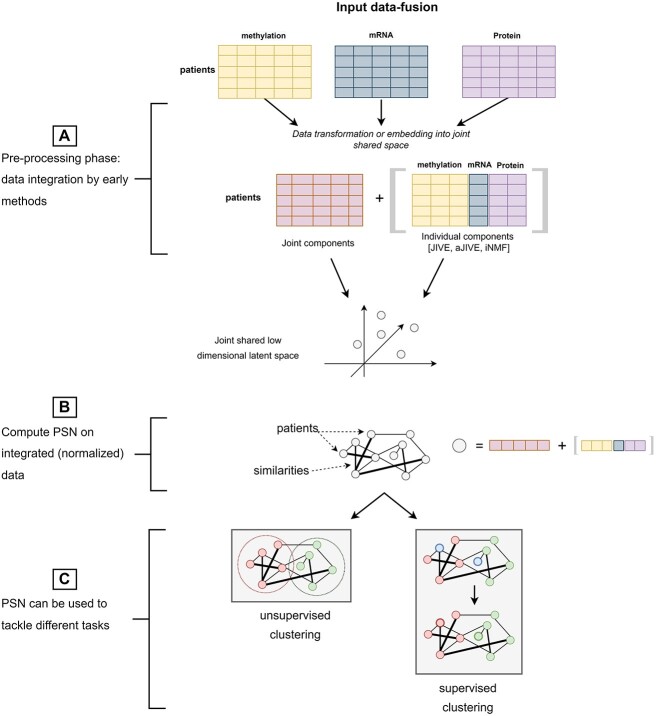
’Input data fusion’ methods are schematized in Figure 3. These approaches are based on the assumption that the input samples originally lied in a latent (eventually orthogonal) space from which the multiple source-views have been generated by unknown projections. This results in data-blocks being expressed into separate source-specific spaces that are characterized by: (1) an individual source-specific structure generating an individual variability within each data-block; (2) a joint sample-specific structure [ref. 18] resulting in shared variance (collinearities) between data-blocks. Therefore, input data-fusion methods estimate the embedding that back-projects the input data-blocks into a shared latent space minimizing redundancy between the data-blocks while maximizing the individual data-block variability. In other words, all the methods find the ’joint components’ (Figure 3) allowing to capture the greatest amount of shared variance; most of the methods also define ways to identify the ’individual components’ capturing the source-specific variability (Figure 3).
Depending on the technique used to project the data into the shared latent space, we can distinguish input data-fusion methods into PCA-based techniques (Table 6) or Matrix Factorization (MF) or Blind Source Separation (BSS)-based methods (Table 7). One advantage of solving the information-fusion in a preprocessing phase, i.e. preceding the construction of an integrated PSN, is that a standard unimodal PSN-analysis model can be subsequently applied (Figure 3B) to deal with clustering or supervised classification problems (Figure 3C). In particular, the input data-fusion methods make the choice of the similarity measure to be used for PSN construction particularly easy, since they compute normalized, a-dimensional, integrated point representations, whose pairwise similarities could be handled by classic measures such as the cosine similarity or the inverted euclidean distance. Moreover, a side-effect of the estimated embedding is that the estimated component loadings or factors may be analyzed for uncovering hidden relationships between variables (data analysis task in Tables 6 and 7 and in Figure 3).
Table 6: PCA-based and CCA-based input data-fusion methods. For each method, the table reports: the name/acronym with the corresponding reference paper; whether it requires the same set of patients across all data modalities (i.e. ‘Matched Samples’); the dataset used to develop and evaluate the approach in the reference paper and the corresponding sample cardinality and data types composing the dataset; the exploited integration method; the application task and the code availability (with link to the repository and programming languages for which the code is available)
| Name | Matched samples | Dataset | Sample cardinality | Data type | Integration approach | Task | Code and Language |
|---|---|---|---|---|---|---|---|
| CPCA [ref. 99] | x | Simulated | Not provided | Numeric | PCA | Data Analysis | |
| CPCA for missing data [ref. 100] | x | Human Mortality Database | 143 | exposure-to-risk | PCA | Data Analysis | |
| (Italy + Switzerland) | |||||||
| JIVE [ref. 18] | x | TCGA BIC | 348 | mRNA | PCA | Unsupervised Clustering (Patient subtype identification) | R code |
| miRNA | |||||||
| methy | |||||||
| RPPA | |||||||
| aJIVE [ref. 97] | x | TCGA extract from | 616 | mRNA | PCA | Data Analysis and | R code |
| [ref. 101] | miRNA | Unsupervised Clustering | |||||
| somatic mutation | (Patient subtype identification) | ||||||
| CNV | |||||||
| RPPA | |||||||
| MCCA [ref. 102] | x | DLBCL Dataset | 203 | mRNA | CCA | Data analysis | R code |
| [ref. 103] | array CGH measurements | ||||||
| RGCCA [ref. 104] | x | SCA Dataset | 67 SCA + | pons volume | CCA | Data Analysis | RGCCA/SGCCA |
| SGCCA [ref. 19] | Private | 35 Healthy | metabolic features | R code | |||
| [ref. 105] | |||||||
| DIABLO [ref. 20] | x | TCGA COAD | 92 | mRNA | (SG)CCA | Data Analysis and | R code |
| TCGA KIRC | 122 | miRNA | Supervised Clustering | ||||
| TCGA GBM | 213 | methy | (Patient’s Survival) | ||||
| TCGA LUSC | 106 | ||||||
| TCGA BRCA | 989 |
CCA: Canonical Correlation Analysis; CGH: Comparative Genomic Hybridization; CNV: Copy Number Variation; DLBCL: Diffuse Large B-Cell Lymphoma; methy: DNA methylation; miRNA: micro RNA; mRNA: messenger RNA; PCA: Principal Component Analysis; RPPA: Reverse Phase Protein Array; SCA: SpinoCerebellar Ataxia; (SG)CCA: (Sparse Generalized) Canonical Correlation Analysis; TCGA+cancer code: The Cancer Genome Atlas+ link to complete cancer codes.
Table 7: MF-based input data-fusion methods. For each method, the table reports: the name/acronym with the corresponding reference paper; whether it requires the same set of patients across all data modalities (i.e. ‘Matched Samples’); the dataset used to develop and evaluate the approach in the reference paper and the corresponding sample cardinality and data types composing the dataset; the exploited integration method; the application task and the code availability (with link to the repository and programming languages for which the code is available). Of note, DFMF [ref. 31] has not been applied to patients’ data but it could be easily adapted to this end.
| Name | Matched samples | Dataset | Sample cardinality | Data type | Integration approach | Task | Code and language |
|---|---|---|---|---|---|---|---|
| MFA | Brain Cancer | Not provided | Multi-omics | MF | Data Analysis | R code | |
| [ref. 107] | Dataset Private | ||||||
| jNMF | x | TCGA OV | 385 | mRNA | NMF | Data Analysis | R code |
| [ref. 121] | miRNA | ||||||
| methy | |||||||
| iNMF | x | TCGA OV | 592 | mRNA | NMF | Unsupervised Clustering | Python code |
| [ref. 98] | miRNA | (Patient subtype identification) | |||||
| methy | |||||||
| iGMFNA | x | TCGA CHOL | 45 | mRNA | NMF | Data Analysis | |
| [ref. 126] | TCGA PAAD | 180 | methy | ||||
| CNV | |||||||
| MOFA+ | Private | Not provided | Multi-omics | NMF | Data Analysis | Python and R code | |
| [ref. 130] | |||||||
| iCluster | x | TCGA CRC | 189 | Exome sequence | NMF | Unsupervised Clustering | R code |
| [ref. 123] | mRNA | (Patient subtype identification) | |||||
| and iCluster+ | methy | ||||||
| [ref. 131] | CNV | ||||||
| DFMF\(}{}$^{3}\) | GO terms | MTF | Unsupervised Clustering | Python code | |||
| [ref. 31] | GO annotations | (hepatotoxic risk associated | |||||
| [ref. 143] | Drugs | with individual drugs) | |||||
| Tissue samples | |||||||
| DILI potentials | |||||||
| MaDDa | TCGA BRCA, | 200 | Gene–gene interactions, | MTF | Unsupervised Clustering (Patient subtype identification) | Matlab code | |
| [ref. 129] | BioGRID | Gene–pathway associations | |||||
| KEGG | Disease–disease relationships, | ||||||
| Disease Ontology | Disease–gene associations, | ||||||
| DisGeNET | Disease–pathway relations | ||||||
| DS-ICA | x | Private | 38 | features from EEG | ICA | Data Analysis | |
| [ref. 142] | and fMRI images | ||||||
| MISA | x | Private | 1001 | EEG images | BSS | Data Analysis | MATLAB code |
| [ref. 21] | sMRI and fMRI images |
BSS: Blind Source Separation; CNV: Copy Number Variation; DILI: Drug-Induced Liver Injury; EEG: Electroencephalography; fMRI: functional Magnetic Resonance Imaging; GO: Gene Ontology; ICA: Independent Component Analysis; KEGG: Kyoto Encyclopedia of Genes and Genomes; methy: DNA methylation; miRNA: micro RNA; MF: Matrix Factorization; mRNA: messenger RNA; MTF: Matrix Tri-Factorization; NMF: Non-negative Matrix Factorization; sMRI: structural Magnetic Resonance Imaging; TCGA+cancer code: The Cancer Genome Atlas+ link to complete cancer codes.
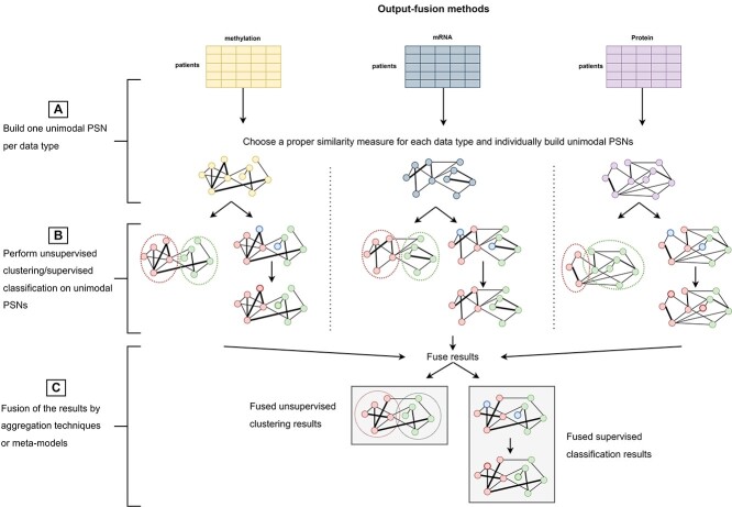
The strategy applied by ’output-fusion’ methods is sketched in Figure 4 and their experimental design is summarized in Table 8. They apply individual PSN pipelines on each data source to obtain individual clustering or supervised prediction results (Figure 4A and B). All the obtained results are then fused by aggregation strategies that, acting as judges, compute a final decision by considering all the individual decisions taken by each unimodal pipeline.
Table 8: Output-fusion methods. For each method, the table reports: the name/acronym with the corresponding reference paper; the dataset used to develop and evaluate the approach in the reference paper and the corresponding sample cardinality and data types composing the dataset; the exploited integration method; the application task and the code availability (with link to the repository and programming languages for which the code is available)
| Name | Dataset | Sample cardinality | Data type | Integration approach | Task | Code and Language |
|---|---|---|---|---|---|---|
| COCA | TCGA AML | 161 | DNA sequence | Consensus Clustering | Unsupervised Clustering | ConsensusClusterPlus |
| [ref. 22] | TCGA BIC | 834 | mRNA | (Patient subtype identification) | R code | |
| TCGA COAD | 182 | miRNA | ||||
| TCGA READ | 73 | methy | ||||
| TCGA GBM | 195 | CNV | ||||
| TCGA KIRC | 475 | RPPA | ||||
| TCGA LUSC | 238 | |||||
| TCGA OV | 329 | |||||
| TCGA UCEC | 345 | |||||
| TCGA BLCA | 120 | |||||
| TCGA LUAD | 270 | |||||
| TCGA HNSC | 305 | |||||
| PINS/PINSPlus | 34 TCGA datasets | 12158 | mRNA | Consensus Clustering | Unsupervised Clustering | R code |
| [ref. 23] | 2 Metabric datasets | miRNA | (Patient subtype identification) | |||
| methy | ||||||
| SUMO | TCGA extract | 3168 across | mRNA | Consensus Clustering | Unsupervised Clustering | Python code |
| [ref. 62] | from NEMO | miRNA | (Patient subtype identification) | |||
| [ref. 94] (Table 4) | methy | |||||
| FH-Clust | TCGA AML | 170 | mRNA | Consensus Clustering | Unsupervised Clustering (Patients’ clusters related to known Survival) | R code |
| [ref. 24] | TCGA BIC | 621 | miRNA | |||
| TCGA COAD | 220 | methy | ||||
| TCGA GBM | 274 | |||||
| TCGA KIRC | 183 | |||||
| TCGA LIHC | 367 | |||||
| TCGA LUSC | 341 | |||||
| TCGA SKCM | 448 | |||||
| TCGA OV | 287 | |||||
| TCGA SARC | 257 | |||||
| [ref. 145] | TCGA KIRC | 418 | Histopathological image | Stacked Generalization: | Supervised Classification | |
| TCGA OV | 250 | RNA-seq data | linear regression of | (Cancer grade < 3 versus Cancer grade >= 3) | ||
| TCGA KIRC | 220 | unimodal classifiers | Supervised Classification | |||
| TCGA OV | 160 | (Known Survival < 5 versus Known Survival >= 5) | ||||
| [ref. 63] | ADNI Phase 1 | 628 for training | Demographic data | Average | Supervised Multiclass classification | Python code |
| [ref. 155] | 94 for validation | APOE e4 allele information | (HC versus MCI versus AD) | |||
| AddNeuroMed study | 88 for testing | anatomical brain features | ||||
| [ref. 156] | from 1.5T MRI scans |
AD: Alzheimer’s Disease; ADNI: Alzheimer’s Disease Neuroimaging Initiative; CNV: Copy Number Variation; HC: Healthy Control; MCI: Mild Cognitive Impairment; methy: DNA methylation; miRNA: micro RNA; MRI: Magnetic Resonance Imaging; mRNA: messenger RNA; RPPA: Reverse-Phase Protein Arrays; TCGA+cancer code: The Cancer Genome Atlas+ link to complete cancer codes.
Input data-fusion via PCA-based and CCA-based methods
In the bioinformatics field, consensus PCA (CPCA [ref. 99]), hierarchical PCA (HPCA [ref. 106]) and Multiple Factor Analysis (MFA [ref. 107]), are some of the most used PCA-based integrative methods. They achieved interesting results on multimodal datasets including different types of patient data, from omics [ref. 18] to images [ref. 108–110].
Their effectiveness is due to their ability to project the data-blocks into a lower dimensional space spanned by not-correlated axis (principal components) maximizing the within-block variances and between-block covariances [ref. 111, ref. 112]. By stretching the data along those axis, they induce a natural separability that improves the performance of the downstream algorithms, which are mostly devoted to data exploration and unsupervised clustering, though some exceptions using supervised clustering exist [ref. 20] (Table 6).
The difference between the three approaches relies on the way the latent space is found. Indeed, while ’CPCA’ solves an optimization problem by an iterative algorithm in the set of nonlinear iterative partial least squares methods (NIPALS [ref. 113]), ’HPCA’ [ref. 106] and ’MFA’ [ref. 107] consecutively apply PCA on respectively: (a) each block separately to derive lower-dimensional ‘stretched’ block representations maximizing the within-block variance; (b) the concatenation of the obtained block representations to derive a stretched latent space maximizing the between-block covariance.
A notable generalization of PCA for multimodal data is ’JIVE’ (Joint and Individual Variation Explained, [ref. 18]), which explicitly models each data-block \(}{}$ {X}_i\) as the sum of a matrix representing the joint structure associated with \(}{}${X}_i\) and shared with other sources, and a matrix representing the source-specific structure characterizing \(}{}$ {X}_i\), and residual noise. Given this formulation, authors apply an iterative estimation procedure that minimizes the reconstruction error, while constraining the axis of the joint and individual structures to be orthogonal (i.e. the joint and individual structures must be uncorrelated). In practice the estimation iterates over the following two steps: (1) having removed the individual structure, apply a sparse singular value decomposition (SVD) to estimate a lower-dimensional joint structure; (2) having removed the joint structure, apply a sparse SVD to find a lower-dimensional individual structure. Interestingly, JIVE also provides a permutation test to select the optimal ranks for the estimated structures. When experimented on multi-omics data from the glioblastoma multiforme (TCGA-GBM) dataset [ref. 18], JIVE showed its ability to effectively uncover the individual and joint data structures, thus leading to a better interpretation of interactions among data types and improving unsupervised classification results. Since the computational complexity of JIVE hampers its applicability, it has been recently reformulated (Angle-Based JIVE—aJIVE [ref. 97]) by using a hierarchical strategy similar to HPCA, which also produces more intuitive interpretations of the obtained decomposition, especially in the presence of strong collinearities. The effectiveness of aJIVE is witnessed by the promising results obtained when applied to an extract of the TCGA breast cancer dataset from [ref. 101] for the (supervised) task of tumor subtype prediction [ref. 114]. In particular the estimated joint components and the first five individual components for each data block are used to compose the integrated sample views to train Random Forest classifiers [ref. 115].
Opposite to PCA-based integrative models, Canonical Correlation Analysis-based (CCA-based) integrative models, e.g. Regularized Generalized CCA (RGCCA) [ref. 104, ref. 105] and its sparse counterpart Sparse Generalized CCA (SGCCA) [ref. 19, ref. 105], find the latent space maximizing the correlation within and between the different data-blocks. They are generally used for exploratory variable analysis since they try to bring all the data blocks to a unique distribution, therefore uncovering hidden relationships between different sources. However, DIABLO [ref. 20] has shown that SGCCA is also effective in the context of supervised clustering for patients’ subtype prediction. In practice, given a multimodal dataset containing \(}{}$N\) samples organized into \(}{}$Y\) classes, DIABLO firstly creates an extra dummy (supervising) data-block where each column is an indicator variable for the point-class (\(}{}$1…Y\)). Next, it uses SGCCA to maximize the covariance between all the data-blocks, including the supervising data-block. Given this representation, supervised clusters may be identified either (1) by averaging the components across data-blocks, to obtain an integrated patient representation that is then used by any supervised clustering algorithm (such as the Maximum Centroids algorithm [ref. 116]); (2) by applying the Maximum Centroids algorithm on each projected data-block to obtain individual clustering results, subsequently aggregated via a majority voting algorithm.
Though effective in several applications, all the aforementioned PCA-based methods suffer from two main limitations: sensitiveness to outliers and inability of handling missing data. Generalized Integrative PCA (GIPCA) [ref. 100] has been recently proposed as an extension of CPCA for dealing with missingness of some values and of entire views. To this aim, eigenvectors are used to explain the intra/inter-block variance by neglecting those samples/views with missing values/views.
Input data-fusion via MF-based methods
MF methods [ref. 117] embed the points into a latent space that minimizes the reconstruction error and whose components (factors) are not constrained to be orthogonal (as in PCA) [ref. 31, ref. 118, ref. 119]. The most effective and used MF method applied on unimodal data is non-negative MF (NMF, [ref. 120]); it constrains both the component and loading matrices to be non-negative, which makes the approximation purely additive.
Given its effectiveness, several works proposed methods where NMF is extended to the integration of multimodal datasets (Table 7). The most relevant example is joint NMF (jNMF [ref. 121]) where multiple NMF problems are solved subject to a shared factor matrix that contains the basis vectors of the shared latent space. However, jNMF is sensitive to random noise and confounding effects [ref. 98] that are specific to each source, and that cannot be detected if a unique shared factor matrix is estimated. This affects the accuracy of the common structure estimation computed by jNMF [ref. 98]. Therefore, integrative non-negative matrix factorization (iNMF [ref. 98]) uses an approach similar to JIVE, where the factor matrices to be estimated are composed both by a shared and a source-specific structure. Unsupervised clustering experiments on the TCGA dataset [ref. 98, ref. 122] have proven the superiority of iNMF with respect to jNMF [ref. 121], NMF [ref. 123] and to integrative Bayesian methods [ref. 124, ref. 125].
Integrative Graph Regularized Non-Negative Matrix Factorization (NMF) for Network Analysis (iGMFNA [ref. 126, ref. 127]) proposes improving the minimization of the reconstruction error, typical of NMF, by exploiting a graph view on each data block. Thanks to such representation, the designed iterative optimization minimizes the reconstruction error while maintaining the topology of the graph views. When compared with jNMF and iNMF to prioritize genes associated with cancer in two TCGA datasets by an unsupervised clustering approach, iGMFNA showed its superior performance.
The popular Penalized Non-negative Matrix Tri-Factorization (NMTF, [ref. 31, ref. 128]) starts from a relational matrix \(}{}${R}_{1,2}\) containing non-negative elements that represent the strengths of the relationships between objects of two different types, \(}{}$\epsilon _1\) and \(}{}$\epsilon _2\), whose respective characteristics are defined by specific constraints, \(}{}${\theta }_1\) and \(}{}${\theta }_2\). NMTF finds the decomposition of \(}{}${R}_{1,2}\), subject to constraints \(}{}${\theta }_1\) and \(}{}${\theta }_2\), such that: \(}{}$ {R}_{1,2} \approx{G}_1 {S}_{1,2} {G}_2^T\) so that \(}{}${G}_1\) and \(}{}$ {G}_2\) are the low-dimensional representations of objects with types, respectively, \(}{}$\epsilon _1\) and \(}{}$\epsilon _2\), and \(}{}$ {S}_{1,2}\) is the backbone matrix linking the two types.
NMTF is exploited by [ref. 31] in Data Fusion by Matrix Factorization (DFMF), where the reliability of the integrated low dimensional estimates computed over a multimodal dataset is improved by considering all the relational matrices (and corresponding constraints) linking the different sources between each other and with the patient data. Given all the relational matrices, \(}{}${R}_{i,j}\), and respective constraints, each \(}{}${R}_{i,j}\) is decomposed so that each backbone matrix represents the latent structure between two data types, the generic low-dimensional data representations of objects with a specific type, \(}{}${G}_i\), is bound to be used in the reconstruction of every relational matrix involving that type. Thanks to the abundance of information, the proposed model can also handle missing data and treat sparse relational matrices. Furthermore, it does not make any assumption about the structural properties of relations, which can also be asymmetric. DFMF can also be used in a semi-supervised setting. During training, the model parameters (i.e. the factorization ranks) are learnt, and are then used in a matrix completion problem, where unobserved entries in the target matrix \(}{}${R}_{i,j}\) are reconstructed for elements that were not present in the training set.
DFMF has been successfully used in the Matrix trifactorization for Discovery of Data similarity and Association (MaDDA) algorithm proposed by [ref. 129] to construct PSNs for unsupervised clustering. In particular, given \(}{}$n\) patients to be partitioned into \(}{}$k\) clusters, the low-rank matrix \(}{}${G} \in{R}^{n \times k}\) estimated through DFMF is viewed as a membership matrix relating each patient to the \(}{}$k\) ranks/groups. After repeating the factorization multiple times with different initialization parameters, a final consensus matrix is obtained by element-wise averaging all membership matrices and then composing a PSN where the similarity between two patients (weight of the edge connecting them) represents how many times they ended up in the same group.
Multi-Omics Factor Analysis+ (MOFA+ [ref. 130]) is an integrative method exploiting Bayesian group factor analysis [ref. 51] with regularization to impose: (i) a view-wise and factor-wise sparsity, which shrinks to zero the loading for the \(}{}$m\)-th modality and the \(}{}$k\)-th factor if the latest does not explain any variability of the \(}{}$m\)-th view; (ii) a feature-wise sparsity, which sets to zero loading on individual features from active factors so that only a small number of features ‘actively’ contribute to each factor. MOFA+ can handle missing values as well as entirely missing views for some samples; moreover, it can cope with heterogeneous data types, which is exactly what is needed when dealing with multimodal datasets containing multi-omics, clinical and imaging data.
Given the successful results of MF-based integrative techniques, some authors have included them as a preprocessing step in their clustering/classification algorithms. As an example, iCluster+ [ref. 123, ref. 131] uses NMF to fuse the heterogeneous data-blocks and then clusters the integrated views. It also exploits the obtained factor loadings to identify the relevant features in the cluster generation.
Input data-fusion via BSS
In their original formulation, BSS models were defined as an extension of NMF techniques for ‘recovering unobservable source signals \(}{}$s\) from measurements \(}{}$x\) (i.e., data), with no knowledge of the parameters \(}{}$\theta\) of the generative system \(}{}$x = f(s, \theta )\)’ [ref. 132].
Given their documented ability [ref. 132–134] of uncovering hidden structures underlying the observed unimodal signals, several BSS models have been extended to handle multimodal datasets comprising also ’multisets’ (Table 7), by a further step that estimates the mixing matrix that recombines all the estimated latent sources so as to compute an integrated, more informative signal with no redundancies [ref. 21, ref. 132, ref. 135, ref. 136]. In particular, multisets are multimodal datasets containing multiple views acquired by the same source under different acquisition conditions (e.g. observation times, experiments, tasks, machines). They are therefore homogeneous [ref. 26] in semantic, type, and dimensionality. Multimodal-multisets are multimodal datasets acquired by different sources, among which sources producing multisets.
Given the lack of information about the mixing process and the source signals, BSS models often differ for the constraints they impose to counter the ill-conditioned problem and obtain essentially unique source estimates [ref. 132, ref. 134, ref. 137]. As an example, the well-known Independent Component Analysis model (ICA [ref. 138]), and its extensions to multimodal data (joint ICA—jICA [ref. 139, ref. 140]), to multisets (Independent Vector Analysis—IVA [ref. 141]) and to multidimensional sources (Independent Subspace Analysis—ISA [ref. 142]), assume a linear (additive) mixture with mutually independent sources and a non-Gaussian distribution of each independent component in the latent space.
All the BSS models base their computations on the existence of collinearities between the observed multimodal data components, so that unreliable results may be obtained when this assumption is not satisfied. Some authors [ref. 135] circumvent this problem by preprocessing the data with CCA (or its multimodal extension), to obtain a projected data representation along correlated components.
The most representative BSS-based multimodal data integration technique is Multidataset Independent Subspace Analysis (MISA [ref. 21, ref. 132]), which was recently proposed to generalize all the BSS models to the fusion of any kind of multimodal-multisets. Motivated by the definition of multiset, MISA is driven by statistical independence between latent subspaces while assuming correspondence within the subspaces underlying the input multisets. In practice, it firstly removes redundancies by estimating nonorthogonal demixing matrices, projecting each multiset into a respective (intermediate) lower-dimensional space spanned by independent components. The sources from all the computed latent spaces are then combined through another demixing matrix that brings all the data-blocks into a unique shared latent space, resulting in an integrated patient view. The de-mixing matrices are estimated by minimizing the mutual information in the final space, while maximizing the mutual information in the intermediate spaces, so as to capture as much correlation as possible. When applied to the integration of the information extracted from functional magnetic resonance imaging (fMRI), structural magnetic resonance imaging (sMRI) and electroencephalogram (EEG) data, MISA has proven its robustness with respect to high signal-to-noise ratios as well as its ability to produce effective data fusion in different ICA contexts.
Output-fusion methods
Following Figure 4, in the context of multimodal PSN analysis the output-fusion methods described in this section may be applied to combine the (unsupervised clustering or supervised classification) results (Figure 4B) computed by individual PSN analyses applied on each data block (see Figure 4A). In Figure 4C, the combination of the unimodal results is performed either by some heuristics, or by majority voting, or by using a meta-model that learns from the predictions performed by each unimodal PSN analysis. Output-fusion techniques have been proposed for clustering samples (mainly from the TCGA datasets, Table 8) to identify patients’ subtypes [ref. 22, ref. 23, ref. 144] and for patients’ classification [ref. 63, ref. 145] (Table 8).
As an example, in Cluster-of-Cluster-Assignments (COCA [ref. 22]), authors combine the clustering results individually obtained by NMF [ref. 146] on each of the six data types of the TCGA datasets. To this aim, the samples are coded into vectors composed of indicator variables representing the clusters they have been assigned in each modality, so that they can be reclustered according to those vectors by Consensus Clustering Plus [ref. 147]. Given the number of clusters \(}{}$k\), Consensus Clustering Plus works on a consensus matrix (\(}{}${CM}_k\)) representing ‘the proportion of clustering runs in which two items are [grouped] together’ [ref. 148]. Given \(}{}${CM}_k\) an agglomerative hierarchical consensus clustering using distance of 1-consensus values is completed and pruned to \(}{}$k\) groups that are returned as consensus clusters.
PINSPlus [ref. 23, ref. 144] similarly exploits Consensus Clustering [ref. 148] for reaching the final partition. In practice, Perturbation clustering for data INtegration and disease Subtyping (PINS) starts by applying any classic unsupervised clustering algorithm (e.g. k-means) individually on each of the \(}{}$M\)-th datasets. If \(}{}$n\) is the number of patients, for the \(}{}$m\)-th dataset (\(}{}$m \in{1, \dots , M}\)) the clustering result is expressed by a square matrix \(}{}${C}_m \in \mathbb{R}^{n \times n}\), such that \(}{}${C}_m(i,j)=1\) if samples \(}{}$i\) and \(}{}$j\) fall in the same cluster, and \(}{}${C}_m(i,j)=0\) otherwise. All the resulting matrices are then averaged to obtain a consensus matrix \(}{}${S} = \frac{\sum _{m = 1}^M {C}_m}{M}\). Even though matrix \(}{}${S}\) may highlight that some points do not reach a strong agreement, authors consider that \(}{}${S}\) itself may be used as a pairwise similarity matrix (since \(}{}${S} = 1\) for points for which there is a strong agreement, viewed as similarity, across all the dataset, and \(}{}${S} = 0\) otherwise) that is suitable for similarity/distance-based clustering algorithms such as any hierarchical Clustering algorithm [ref. 149], Partitioning Around Medoids [ref. 150] or dynamic tree cut [ref. 151]. In their work, authors propose testing different clustering algorithms and then choose the partition that agrees the most with the partitioning of individual data types.
Consensus clustering has also been successfully applied by the recently published SUMO [ref. 62], an integrative clustering algorithm that starts by computing several unimodal PSNs by using a scaled-normalized Euclidean kernel similar to the one exploited by SNF [ref. 3]. SUMO then formulates a constrained NMTF (see Section Input data-fusion via MF-based methods) to find a sparse shared representation of all the samples in the cluster subspace by accounting for the adjacencies observed in all the data types. The NMTF optimization problem is solved by an iterative procedure that is applied several times on several sample subsets to ensure robustness with respect to the initial conditions and to the input data; consensus clustering is then exploited to pool together the clustering results. When compared with the most promising integrative clustering methods (e.g. iCluster [ref. 152], Multiple Canonical Correlation Analysis (MCCA) [ref. 102], NEMO [ref. 94], SNF [ref. 3], PINSPlus [ref. 23]) SUMO obtained impressive results.
The Fuzzy-hierarchical CLUSTering—FH-Clust method [ref. 24] interestingly proposes to use fuzzy logic for identifying patients’ prognostic subgroups from multiomics data, resting on the fact that in nature there is often no clear cut between subtypes. Unimodal data are separately analyzed using a fuzzy-based hierarchical clustering approach exploiting a Lukasiewicz valued fuzzy similarity and individual results are then fused through a consensus matrix. Extensive experiments on 10 cancer datasets from TCGA (considering gene expression, miRNA, methylation data) show that FH-Clust is competitive with state-of-the-art methods (i.e. k-means, Spectral Clustering, LRACluster, PINS, SNF, MCCA).
Interesting output-fusion approaches aimed at patients’ classification are described in [ref. 63, ref. 145]. In [ref. 145] the authors obtain effective cancer-grade and patient-survival classifications for cancer patients represented in the TCGA renal (TCGA KIRC) and TCGA ovarian (TCGA OV) datasets by using all the data types included in TCGA, including hematoxylin and eosin (H&E)-stained whole-slide images of tissue samples that are processed by digital image processing techniques to extract more that 400 features per sample. In practice authors firstly individually process each data block to apply an internal cross-validation approach to choose (1) the number of informative features to be extracted by the minimum Redundancy Maximum Relevance (mRMR) method [ref. 153] and (2) the best performing 5-fold cross classifier among SVM, logistic regression, K-nearest neighbors and Linear Discriminant Analysis. To compose all the predictions from the different modalities authors compare the stacked generalization model [ref. 154], which essentially trains a logistic regression classifier on the obtained predictions, to the majority vote strategy. The best results are obtained by the stacked prediction model, which leverages the results obtained by any of the multimodal predictions, independent from the classifier that is used for producing them.
In [ref. 63] authors simply use the average to integrate the different prognostic classifications computed over multimodal profiles of suspected Alzheimer Disease (AD) patients, with the aim of identifying patients who are vulnerable to conversion from mild-cognitive impairment to AD. In particular, the squared-exponential kernels are firstly used to build unimodal PSNs, and, for each unimodal network, a Gaussian process is then exploited to assign labels to unknown points based on the nearest known points. Finally, the unknown patients’ condition is computed as the average over all the unimodal predictions.
Discussion and conclusion
In the context of precision medicine, PSNs are gaining momentum given their ability to uncover and exploit relationships among patients when applied to clustering and classification tasks [ref. 9]. According to the state-of-the-art surveys describing the application of PSNs for precision medicine or health data processing [ref. 9, ref. 45, ref. 157, ref. 158], PSN-based models benefit from several advantages; they are: (1) easy to understand, (2) interpretable by design, (3) privacy preserving, (4) competitive or even superior to state-of-the-art clustering/classification methods, (5) potentially able to integrate different data views. In particular, the possibility of using PSN models in a multimodal setting is especially relevant in light of the increasing availability of digital technologies by means of which huge amount of multimodal data can be collected that describe each patient/sample by considering different biological/medical views. Moreover, in the past few years the increasing availability of cloud technologies allowed us to distribute data processing across multiple local servers belonging to, e.g. different institutions. In this context, the development of promising information integration models would allow the application of a Federated Learning strategy [ref. 159], where a central server collects, further integrates, and eventually processes, the (already) integrated data, or the individual PSNs, or the predictions individually computed by local servers located in the institutions where the data belong. In this way, the initial processing of the sensitive data would be demanded to the local institutions to protect patient privacy, and the central server would have access only to preprocessed information, thus hiding explicit sensitive data.
Though in the biomedical context several multimodal approaches have already shown their ability to integrate multimodal data to improve the results obtained from a single view (unimodal data) [ref. 114], and the survey literature about data integration methods for multimodal data is wide [ref. 13, ref. 15, ref. 16], in the field of PSN analysis only few methods have already investigated the usage of multimodal data, by building integrated PSNs that exploit both the joint and the individual information from all the available sources. Moreover, no state-of-the-art survey has focused on the role of PSN as a cornerstone for data fusion. In this survey, we aim at filling this gap with the goal of providing interested readers with a comprehensive collection of integrative methods that may be exploited to build PSN approaches efficiently handling multimodal data.
Besides an extensive literature search, the integration approaches have been organized into three broad classes on the basis of the type of data that is fused: ’PSN-fusion’, ’Input data-fusion’ and ’Output-fusion’ methods. More precisely, ’PSN-fusion’ methods may be split into the three sub-classes of ’MKL’, ’SNF-based’ and ’other’ methods, whereas ’Input data-fusion’ approaches comprehend algorithms ’PCA-based’, ’CCA-based’ and ’MF-based’.
The survey has highlighted the promising results and advantages that characterize the methods belonging to the three classes of our proposed taxonomy.
Methods based on PSN-fusion techniques are particularly useful in network medicine applications [ref. 160] that study human diseases through ‘systemic’ approaches in which diseases are interpreted as perturbations in complex biomolecular networks. In this context, transductive strategies working on individual PSN models [ref. 7] would benefit from the application of PSN-fusion approaches, as shown by recent promising results [ref. 3, ref. 6].
Methods based on input-data fusion techniques rely on factor analysis models for the removal of data collinearities and the simultaneous enhancement of the individual structure characterizing each view. For this reason, we believe such techniques are particularly useful when dealing with multiview data involving follow-up examinations, where the multiple views likely contain correlated information.
Output-fusion techniques should be used when the differences between the multimodal views impose the usage of peculiar and specific unimodal PSN models for obtaining individual inferences. This is the case, for example when we need to combine data having substantially different structures, ranging from vectorial to sequence and graph-structured data.
Though being effective, our thorough review also evidenced difficulties and drawbacks that harbour from the data-fusion strategy. In particular, PSN-fusion models require to build an individual PSNs on each data type. This raises the crucial, still open, and often overlooked problem of choosing proper individual similarity measures for building each unimodal PSNs. Indeed, only few methods [ref. 60, ref. 161, ref. 162] reported exhaustive comparative evaluations among few distance metrics applied to genetic data. By considering that several problems in precision medicine are characterized by nonlinearly separable omics data, and given the experimental results we have collected during our literature search, we recommend computing PSNs by exploiting a kernel function. In this context, though several functions have been successfully proposed and used in literature, when dealing with continuous data, we suggest using the scaled exponential kernel of Euclidean distance [ref. 3, ref. 62], due to its ability to adapt to different neighborhood sizes. This allows dealing with datasets distributed on complex manifolds where datapoints are not evenly distributed in space, as it often happens in real-world problems. On the other hand, when dealing with simpler data types with lower dimensionalities and complexities (e.g. clinical data), simpler normalized similarities may be sufficient to appropriately capture the data structure. Clinical datasets usually contain categorical variables, often mixed with numeric features. The former situation can be appropriately addressed by averaging the normalized similarities individually computed on each variable [ref. 6], whereas Chi-squared distances are the most suitable for categorical data [ref. 3, ref. 6]. Of note, the subsequent application of a Random Walk kernel, as proposed by Gliozzo et al. [ref. 7], is a promising step to refine the obtained PSN.
On the other side, input data-fusion techniques integrate the input data by projecting them into a shared space with lower dimensionality, thus making these approaches strongly dependent on the chosen final dimensionality \(}{}$d\).
While classic approaches have been proposed to automatically set \(}{}$d\) [ref. 100, ref. 163–165], this value is often user-defined after observation of the scree plot. However, observing that the optimal latent vector space is the one that allows to capture the intrinsic data structure, we instead suggest setting \(}{}$d\) to the intrinsic data dimensionality (id) [ref. 166], which is the minimum number of parameters needed to represent the data without information loss.
Finally, output-data fusion methods are often too generic or use very simple output-aggregation strategies, e.g. average or majority voting, that may produce suboptimal results.
Generally speaking, our survey evidenced some important open issues in the context of data integration methods for PSN that call for the future research directions summarized in the following subsection.
Future research directions
While conducting our survey we noted the need of investigating methods for data pre-processing, with the aim of, e.g. detecting and eliminating noise with heterogeneous characteristics, collinearities between different views, and confoundings that could bias the final results (as per [ref. 27]). Indeed, only few recently proposed preliminary attempts were able to explicitly consider the presence of noise with heterogeneous characteristics [ref. 98, ref. 122].
Moreover, future research should be devoted to the investigation of novel multimodal feature-selection algorithms. Indeed, the few methods applying a feature selection step exploit either classic univariate statistics, or algorithms, such as mRMR [ref. 153], that analyze group of features by neglecting their multimodal characteristics.
On the other side, missing data imputation needs deeper investigation to handle two types of biomedical data-missingness: (1) missingness of some data values in some views; (2) missingness of entire views for some samples. While missingness is becoming a common problem in different fields, in the biomedical field few approaches present thorough missing data imputation studies [ref. 11]. Besides, among the approaches we have surveyed, only GIPCA [ref. 100] specifically addressed both these types of missingness. Finally, given the big-data produced by high-throughput technologies, scalability is becoming an important and often overlooked issue, nowadays hampering the applicability of several promising tools.
Though the aforementioned issues are still open, all the surveyed strategies have reported promising results that might improve knowledge in then field of precision medicine. Unfortunately, different similarity metrics, experimental setups and evaluation measures are used for model assessment; this hampers an objective comparison between the different integration techniques and data analysis models. Furthermore, we found no evidence about data integration approaches that should be preferred over the others. Instead, the type and semantic of the available data type and the specific biomedical question to address should guide the choice. An additional open problem regards the identification of the most appropriate similarity/distance measure for each biological data modality. To the best of our knowledge, only few works tried to investigate this issue by comparing different metrics for specific data views and most of them are focused on gene expression data [ref. 60, ref. 161, ref. 162]. Comprehensive studies comparing the usage of different similarity measures in different contexts (e.g. when applied to different biological data types and in supervised and unsupervised prediction contexts) would provide fruitful insights to guide the scientific community towards effective PSN construction. We also remark that, though some algorithms are already available as open source packages/repositories (mostly coded using R, Python and Matlab) [ref. 16], many others are not, thus slowing down their diffusion and testing by the community.
Another interesting research line that should be given attention is represented by the development of Web applications extending, e.g. those presented in [ref. 167, ref. 168], for the visual analysis of PSN models. Indeed, the graphical tools can enable the visual comparison of different PSN models realized according to any of the methods discussed in this survey. This in turn can improve the explainability of the computed results and would allow the user to choose the approach mostly suited to her/his needs.
Author contributions statement
J.G., G.V. and E.C. conceived the work, J.G. collected the literature papers, J.G. and E.C. studied the literature, selected the most relevant works and drafted them; J.G, M.M., M.N., A.Pac., G.V., E.C. wrote the paper; all the authors validated the work.
Key Points
- Patients similarity networks (PSN) are explainable and privacy preserving representations of patients that leverage the similarity of their clinical/biomolecular profiles to construct graphs of patients.
- Network Medicine algorithms on PSNs for patient stratification, phenotype and outcome prediction and disease risk assessment represent novel tools for Genomic and Precision Medicine
- The combination of clinical, omics and imaging bio-medical data can lead to novel PSNs able to leverage the synergy of multiple views of the patients.
- Several reviews about data integration methods in bioinformatics and biomedical applications have been proposed but no specific reviews about the emerging field of heterogeneous data integration methods for patient similarity networks are actually available.
- We provide a thorough review and propose a taxonomy of heterogeneous data integration methods for PSNs, together with the different patient similarity measures proposed in literature.
- We also review methods that have appeared in the machine learning literature but have not yet been applied to PSNs, thus providing a resource to navigate the vast machine learning literature existing on this topic.
- Strengths and limitations of the proposed methods are discussed to both assist researchers in the design and development of novel methods and to guide the selection of PSN integration methods for specific applications, focusing on methods that could be used to integrate very diverse datasets, including multi-omics data as well as data derived from clinical information and medical imaging.
References
- What is precision medicine?. Eur Respir J, 2017
- Building the foundation for genomics in precision medicine.. Nature, 2015. [PubMed]
- Similarity network fusion for aggregating data types on a genomic scale.. Nat Methods, 2014. [PubMed]
- Knowledge boosting: a graph-based integration approach with multi-omics data and genomic knowledge for cancer clinical outcome prediction.. J Am Med Inform Assoc, 2015. [PubMed]
- Identification of type 2 diabetes subgroups through topological analysis of patient similarity.. Sci Transl Med, 2015
- netdx: interpretable patient classification using integrated patient similarity networks.. Mol Syst Biol, 2019. [PubMed]
- Network modeling of patients’ biomolecular profiles for clinical phenotype/outcome prediction.. Sci Rep, 2020. [PubMed]
- Integrated multi-omics analyses in oncology: a review of machine learning methods and tools.. Front Oncol, 2020. [PubMed]
- Patient similarity networks for precision medicine.. J Mol Biol, 2018. [PubMed]
- Precision medicine-a promising, yet challenging road lies ahead.. Curr Opin Syst Biol, 2018
- Explainable machine learning for early assessment of Covid-19 risk prediction in emergency departments.. IEEE Access, 2020. [PubMed]
- A survey on mining multiple data sources.. Wiley Interdiscip Rev Data Min Knowl Discov, 2013
- Methods for the integration of multi-omics data: mathematical aspects.. BMC Bioinf, 2016
- Integrative methods for analyzing big data in precision medicine.. Proteomics, 2016. [PubMed]
- Dimension reduction techniques for the integrative analysis of multi-omics data.. Brief Bioinform, 2016. [PubMed]
- Multi-omics data integration, interpretation, and its application.. Bioinform Biol Insights, 2020. [PubMed]
- Simplemkl.. J Mach Learn Res, 2008
- Joint and individual variation explained (jive) for integrated analysis of multiple data types.. Ann Appl Stat, 2013. [PubMed]
- Variable selection for generalized canonical correlation analysis.. Biostatistics, 2014. [PubMed]
- Diablo: an integrative approach for identifying key molecular drivers from multi-omics assays.. Bioinformatics, 2019. [PubMed]
- Multidataset independent subspace analysis with application to multimodal fusion.. IEEE Trans Image Process, 2020. [PubMed]
- Multiplatform analysis of 12 cancer types reveals molecular classification within and across tissues of origin.. Cell, 2014. [PubMed]
- Pinsplus: a tool for tumor subtype discovery in integrated genomic data.. Bioinformatics, 2019. [PubMed]
- Data integration by fuzzy similarity-based hierarchical clustering.. BMC Bioinf, 2020
- A selective review of multi-level omics data integration using variable selection.. High-Throughput, 2019
- Methods for biological data integration: perspectives and challenges.. J R Soc Interface, 2015. [PubMed]
- Methods of integrating data to uncover genotype–phenotype interactions.. Nat Rev Genet, 2015. [PubMed]
- Multimodal machine learning: a survey and taxonomy.. IEEE Trans Pattern Anal Mach Intell, 2018. [PubMed]
- Learning gene functional classifications from multiple data types.. J Comput Biol,, 2002. [PubMed]
- 30. Daemen A, Gevaert O, De Moor B. Integration of clinical and microarray data with kernel methods. In: 2007 29th Annual International Conference of the IEEE Engineering in Medicine and Biology Society. Piscataway, New Jersey, United States: IEEE, 2007, 5411–5.
- Data fusion by matrix factorization.. IEEE Trans Pattern Anal Mach Intell, 2014
- A review on machine learning principles for multi-view biological data integration.. Brief Bioinform, 2018. [PubMed]
- A survey on single and multi omics data mining methods in cancer data classification.. J Biomed Inform, 2020. [PubMed]
- 34. Tang W, Zhengdong L, Dhillon IS. Clustering with multiple graphs. In: Wei Wang, Hillol Kargupta, Sanjay Ranka, Philip S. Yu, Xindong Wu (eds.) 2009 Ninth IEEE International Conference on Data Mining. Piscataway, New Jersey, United States: IEEE, 2009, 1016–21.
- Integration of clinical and gene expression data has a synergetic effect on predicting breast cancer outcome.. PLoS One, 2012. [PubMed]
- A statistical framework for genomic data fusion.. Bioinformatics, 2004. [PubMed]
- Predicting the prognosis of breast cancer by integrating clinical and microarray data with Bayesian networks.. Bioinformatics, 2006. [PubMed]
- Moli: multi-omics late integration with deep neural networks for drug response prediction.. Bioinformatics, 2019. [PubMed]
- On the similarity metric and the distance metric.. Theor Comput Sci, 2009
- 40. Belanche L, Orozco J. Things to know about a (dis) similarity measure. In: Koenig A, Dengel A, Hinkelmann K, Kise K, Howlett RJ, Jain LC (eds.) International Conference on Knowledge-Based and Intelligent Information and Engineering Systems. Berlin, Heidelberg: Springer, 2011, 100–9.
- 41. Schölkopf B, Smola A, Müller K-R. Kernel Principal Component Analysis. In: Wulfram Gerstner, Alain Germond, Martin Hasler, Jean-Daniel Nicoud (eds.) International Conference on Artificial Neural Networks. Berlin, Heidelberg: Springer, 1997, 583–8.
- A survey on graph kernels.. Appl Netw Sci, 2020
- An experimental investigation of kernels on graphs for collaborative recommendation and semisupervised classification.. Neural Netw, 2012. [PubMed]
- Personalized mortality prediction driven by electronic medical data and a patient similarity metric.. PLoS One, 2015. [PubMed]
- Patient similarity in prediction models based on health data: a scoping review.. JMIR Med Inform, 2017. [PubMed]
- Towards personalized medicine: leveraging patient similarity and drug similarity analytics.. AMIA Summits Trans Sci Proc, 2014
- A survey of binary similarity and distance measures.. J Syst Cybern Inf, 2010
- 48. Klenk S, Dippon J, Fritz P, et al. Determining patient similarity in medical social networks. In: Proceedings of the First International Workshop on Web Science and Information Exchange in the Medical Web, 2010, 6–14.
- 49. Schölkopf B . The kernel trick for distances. In: Todd K. Leen, Thomas G. Dietterich and Volker Tresp (eds.) Advances in neural information processing systems. A Bradford Book, 2001, 301–7.
- Integrating clinical and multiple omics data for prognostic assessment across human cancers.. Sci Rep, 2017. [PubMed]
- Improve glioblastoma multiforme prognosis prediction by using feature selection and multiple kernel learning.. IEEE/ACM Trans Comput Biol Bioinform, 2016. [PubMed]
- Unsupervised multiple kernel learning for heterogeneous data integration.. Bioinformatics, 2018. [PubMed]
- Improved modeling of clinical data with kernel methods.. Artif Intell Med, 2012. [PubMed]
- Using association signal annotations to boost similarity network fusion.. Bioinformatics, 2019. [PubMed]
- Kernel fusion method for detecting cancer subtypes via selecting relevant expression data.. Front Genet, 2020
- RANKS: a flexible tool for node label ranking and classification in biological networks.. Bioinformatics, 06 2016. [PubMed]
- Pamogk: a pathway graph kernel based multi-omics approach for patient clustering.. Bioinformatics, 2020
- Multi-dimensional data integration algorithm based on random walk with restart.. BMC Bioinf, 2021
- Proximity measures for clustering gene expression microarray data: a validation methodology and a comparative analysis.. IEEE/ACM Trans Comput Biol Bioinform, 2013. [PubMed]
- On the selection of appropriate distances for gene expression data clustering.. BMC Bioinf, 2014
- Integrative gene network construction to analyze cancer recurrence using semi-supervised learning.. PLoS One, 2014
- Detecting molecular subtypes from multi-omics datasets using sumo.. Cell Rep Methods, 2022. [PubMed]
- A similarity-based approach to leverage multi-cohort medical data on the diagnosis and prognosis of Alzheimer’s disease.. GigaSci, 2018
- Multiple kernel learning in the primal for multimodal Alzheimer’s disease classification.. IEEE J Biomed Health Inform, 2013. [PubMed]
- Classifying breast cancer subtypes using multiple kernel learning based on omics data.. Genes, 2019
- Multiple kernel learning algorithms.. J Mach Learn Res, 2011
- A novel MKL method for GBM prognosis prediction by integrating histopathological image and multi-omics data.. IEEE J Biomed Health Inform, 2019. [PubMed]
- Support vector machines and kernel methods: the new generation of learning machines.. Ai Mag, 2002
- Integrating genomic data and pathological images to effectively predict breast cancer clinical outcome.. Comput Methods Programs Biomed, 2018. [PubMed]
- Easymkl: a scalable multiple kernel learning algorithm.. Neurocomputing, 2015
- 71. Xu Z, Jin R, Yang H, et al. Simple and efficient multiple kernel learning by group lasso. In: Johannes Fürnkranz,Thorsten Joachims (eds.) Proceedings of the 27th international conference on machine learning (ICML-10). Omnipress, 2600 Anderson St, Madison, WI, United States: Citeseer, 2010, 1175–82.
- Spicymkl: a fast algorithm for multiple kernel learning with thousands of kernels.. Mach Learn, 2011
- Non-sparse multiple kernel fisher discriminant analysis.. J Mach Learn Res, 2012
- Generalized discriminant analysis using a kernel approach.. Neural Comput, 2000. [PubMed]
- 75. Ong CS, Zien A. An automated combination of kernels for predicting protein subcellular localization. In: Keith A. Crandall, Jens Lagergren (eds.) International Workshop on Algorithms in Bioinformatics. Berlin, Heidelberg: Springer, 2008, 186–97.
- Integrating different data types by regularized unsupervised multiple kernel learning with application to cancer subtype discovery.. Bioinformatics, 2015. [PubMed]
- 77. Liu X, Dou Y, Yin J, et al. (eds). Multiple kernel k-means clustering with matrix-induced regularization. In: Proceedings of the AAAI Conference on Artificial Intelligence, 2016.
- Multiple kernel learning for dimensionality reduction.. IEEE Trans Pattern Anal Mach Intell, 2011. [PubMed]
- Locality preserving projections.. Adv Neural Inform Process Syst, 2004
- Nonlinear component analysis as a kernel eigenvalue problem.. Neural Comput, 1998
- An extensive analysis of disease-gene associations using network integration and fast kernel-based gene prioritization methods.. Artif Intell Med, 2014. [PubMed]
- 82. Pearl J . Probabilistic reasoning in intelligent systems: networks of plausible inference. Elsevier, 2014.
- Multi-omics integration-a comparison of unsupervised clustering methodologies.. Brief Bioinform, 2019. [PubMed]
- Systems proteomics of liver mitochondria function.. Science, 2016
- New molecular insights into modulation of platelet reactivity in aspirin-treated patients using a network-based approach.. Hum Genet, 2016. [PubMed]
- Comprehensive molecular portraits of human breast tumours.. Nature, 2012. [PubMed]
- 87. Ma T, Zhang A. Integrate multi-omic data using affinity network fusion (ANF) for cancer patient clustering. In 2017 IEEE International Conference on Bioinformatics and Biomedicine (BIBM), pages 398–403. IEEE, 2017.
- Novel fisher discriminant classifiers.. Pattern Recognit, 2012
- 89. Liu S, Shang X. Hierarchical similarity network fusion for discovering cancer subtypes. In: Fa Zhang, Zhipeng Cai, Pavel Skums, Shihua Zhang (eds.) International Symposium on Bioinformatics Research and Applications. Cham, Switzerland: Springer, 2018, 125–36.
- Discovering cancer subtypes via an accurate fusion strategy on multiple profile data.. Front Genet, 2019. [PubMed]
- Multilayer networks.. J Complex Netw, 2014
- Random walk with restart on multiplex and heterogeneous biological networks.. Bioinformatics, 2019. [PubMed]
- Multi-omic and multi-view clustering algorithms: review and cancer benchmark.. Nucleic Acids Res, 2018. [PubMed]
- Nemo: Cancer subtyping by integration of partial multi-omic data.. Bioinformatics, 2019. [PubMed]
- Multi-view spectral clustering based on multi-smooth representation fusion for cancer subtype prediction.. Front Genet, 2021
- 96. Nie F, Li J, Li X, et al. Self-weighted multiview clustering with multiple graphs. In: Carles Sierra (ed.) IJCAI. International Joint Conferences on Artificial Intelligence, 2017, 2564–70.
- Angle-based joint and individual variation explained.. J Multivariate Anal, 2018
- A non-negative matrix factorization method for detecting modules in heterogeneous omics multi-modal data.. Bioinformatics, 2016. [PubMed]
- Analysis of multiblock and hierarchical PCA and PLS models.. J Chemometr, 1998
- Generalized integrative principal component analysis for multi-type data with block-wise missing structure.. Biostatistics, 2020. [PubMed]
- Comprehensive molecular portraits of invasive lobular breast cancer.. Cell, 2015. [PubMed]
- Extensions of sparse canonical correlation analysis with applications to genomic data.. Stat Appl Genet Mol Biol, 2009
- Molecular subtypes of diffuse large b-cell lymphoma arise by distinct genetic pathways.. Proc Natl Acad Sci, 2008. [PubMed]
- Regularized generalized canonical correlation analysis.. Psychometrika, 2011
- A strategy for multimodal data integration: application to biomarkers identification in spinocerebellar ataxia.. Brief Bioinform, 2018. [PubMed]
- A framework for sequential multiblock component methods.. J Chemometr, 2003
- Simultaneous analysis of distinct omics data sets with integration of biological knowledge: multiple factor analysis approach.. BMC Genomics, 2009. [PubMed]
- Integration of multimodal MRI data via PCA to explain language performance.. NeuroImage, 2014. [PubMed]
- Dimensionality reduction of diffusion mri measures for improved tractometry of the human brain.. Neuroimage, 2019. [PubMed]
- Multimodal principal component analysis to identify major features of white matter structure and links to reading.. PLoS ONE., 2020. [DOI]
- A sequential algorithm for multiblock orthogonal projections to latent structures.. Chemom Intel Lab Syst, 2015
- Deep learning-based multi-omics data integration reveals two prognostic subtypes in high-risk neuroblastoma.. Front Genet, 2018. [PubMed]
- PLS-regression: a basic tool of chemometrics.. Chemom Intel Lab Syst, 2001
- Integrative, multi-omics, analysis of blood samples improves model predictions: applications to cancer.. BMC Bioinformatics, 2021. [DOI]
- Random forests.. Mach Learn, 2001
- mixomics: an r package for ‘omics feature selection and multiple data integration.. PLoS Comput Biol, 2017. [PubMed]
- Comparison of dimension reduction techniques in the analysis of mass spectrometry data.. Atmos Meas Tech, 2020
- Sparse and unique nonnegative matrix factorization through data preprocessing.. J Mach Learn Res, 2012
- 119. Li Y . Advances in multi-view matrix factorizations. In: 2016 International Joint Conference on Neural Networks (IJCNN). Piscataway, New Jersey, United States: IEEE, 2016, 3793–800.
- Non-negative matrix factorization with sparseness constraints.. J Mach Learn Res, 2004
- Discovery of multi-dimensional modules by integrative analysis of cancer genomic data.. Nucleic Acids Res, 2012. [PubMed]
- Evaluation of integrative clustering methods for the analysis of multi-omics data.. Brief Bioinform, 2020. [PubMed]
- Integrative clustering of multiple genomic data types using a joint latent variable model with application to breast and lung cancer subtype analysis.. Bioinformatics, 2009. [PubMed]
- Bayesian consensus clustering.. Bioinformatics, 2013. [PubMed]
- Bayesian correlated clustering to integrate multiple datasets.. Bioinformatics, 2012. [PubMed]
- An integrated graph regularized non-negative matrix factorization model for gene co-expression network analysis.. IEEE Access, 2019
- Graph regularized nonnegative matrix factorization for data representation.. IEEE Trans Pattern Anal Mach Intell, 2010. [PubMed]
- 128. Wang F, Li T, Zhang C. Semi-supervised clustering via matrix factorization. In: Chid Apte, Haesun Park, Ke Wang, and Mohammad J. Zaki (eds.) Proceedings of the 2008 SIAM International Conference on Data Mining (SDM), 2008, pp. 1–12.
- Patient similarity by joint matrix trifactorization to identify subgroups in acute myeloid leukemia.. JAMIA Open, 2018. [PubMed]
- Mofa+: a statistical framework for comprehensive integration of multi-modal single-cell data.. Genome Biol, 2020
- Pattern discovery and cancer gene identification in integrated cancer genomic data.. Proc Natl Acad Sci, 2013. [PubMed]
- Blind source separation for unimodal and multimodal brain networks: a unifying framework for subspace modeling.. IEEE J Selected Topics Signal Process, 2016
- Learning the parts of objects by non-negative matrix factorization.. Nature, 1999. [PubMed]
- Linked component analysis from matrices to high-order tensors: applications to biomedical data.. Proc IEEE, 2016
- Diversity in independent component and vector analyses: Identifiability, algorithms, and applications in medical imaging.. IEEE Signal Process Mag, 2014
- Multimodal data fusion: an overview of methods, challenges, and prospects.. Proc IEEE, 2015
- 137. Comon P, Jutten C. In: P. Comon, C. Jutten (eds.) Handbook of Blind Source Separation: Independent Component Analysis and Applications. Cambridge, Massachusetts, United States: Academic Press, 2010.
- Independent component analysis: algorithms and applications.. Neural Netw, 2000. [PubMed]
- 139. Calhoun V, Adali T, Liu J. A feature-based approach to combine functional MRI, structural MRI and EEG brain imaging data. In: 2006 International Conference of the IEEE Engineering in Medicine and Biology Society. Piscataway, New Jersey, United States: IEEE, 2006, 3672–5.
- Joint independent component analysis for simultaneous EEG–fMRI: principle and simulation.. Int J Psychophysiol, 2008. [PubMed]
- 141. Kim T, Eltoft T, Lee T-W. Independent vector analysis: an extension of ICA to multivariate components. In: Justinian Rosca, Deniz Erdogmus, José C. Príncipe, Simon Haykin (eds.) International conference on independent component analysis and signal separation. Berlin, Heidelberg: Springer, 2006, 165–72.
- ICA and IVA for data fusion: an overview and a new approach based on disjoint subspaces.. IEEE Sensors Lett, 2018
- Matrix factorization-based data fusion for drug-induced liver injury prediction.. Syst Biomed, 2014
- A novel approach for data integration and disease subtyping.. Genome Res, 2017. [PubMed]
- 145. Phan JH, Hoffman R, Kothari S, et al. Integration of multi-modal biomedical data to predict cancer grade and patient survival. In: 2016 IEEE-EMBS International Conference on Biomedical and Health Informatics (BHI). Piscataway, New Jersey, United States: IEEE, 2016, 577–80.
- Metagenes and molecular pattern discovery using matrix factorization.. Proc Natl Acad Sci, 2004. [PubMed]
- Consensusclusterplus: a class discovery tool with confidence assessments and item tracking.. Bioinformatics, 2010. [PubMed]
- Consensus clustering: a resampling-based method for class discovery and visualization of gene expression microarray data.. Mach Learn, 2003
- Algorithms for hierarchical clustering: an overview.. Wiley Interdiscip Rev Data Min Knowl Discov, 2012
- Clustering by means of medoids.. Data Anal Based L1-Norm Related Methods, 1987
- Defining clusters from a hierarchical cluster tree: the dynamic tree cut package for r.. Bioinformatics, 2008. [PubMed]
- Fast dimension reduction and integrative clustering of multi-omics data using low-rank approximation: application to cancer molecular classification.. BMC Genomics, 2015. [PubMed]
- Minimum redundancy feature selection from microarray gene expression data.. J Bioinform Comput Biol, 2005. [PubMed]
- Stacked generalization.. Neural Netw, 1992
- The Alzheimer’s disease neuroimaging initiative (ADNI): MRI methods.. J Magn Reson Imaging, 2008. [PubMed]
- Addneuromed-the European collaboration for the discovery of novel biomarkers for Alzheimer’s disease.. Ann N Y Acad Sci, 2009. [PubMed]
- Patient similarity: emerging concepts in systems and precision medicine.. Front Physiol, 2016. [PubMed]
- Patient similarity: methods and applications.. 2020
- Federated learning for healthcare informatics.. J Healthc Inf Res, 2021
- Network medicine: a network-based approach to human disease.. Nat Rev Genet, 2011. [PubMed]
- 161. Giancarlo R, Bosco GL, Pinello L. Distance functions, clustering algorithms and microarray data analysis. In: Christian Blum, Roberto Battiti (eds.) International Conference on Learning and Intelligent Optimization. Berlin, Heidelberg: Springer, 2010, 125–38.
- Impact of similarity metrics on single-cell RNA-seq data clustering.. Brief Bioinform, 2019. [PubMed]
- Principal component analysis: a beginner’s guide-II. Pitfalls, myths and extensions.. Weather, 1993
- Selecting the number of principal components: Estimation of the true rank of a noisy matrix.. Ann Stat, 2017
- A general framework for association analysis of heterogeneous data.. Ann Appl Stat, 2018
- Intrinsic dimension estimation: relevant techniques and a benchmark framework.. Math Probl Eng, 2015
- Unipred-web: a web tool for the integration and visualization of biomolecular networks for protein function prediction.. BMC Bioinf, 2019
- Multi-resolution visualization and analysis of biomolecular networks through hierarchical community detection and web-based graphical tools.. PLoS One, 12 2020
- Statistical methods in integrative genomics.. Annu Rev Stat Appl, 2016. [PubMed]
- Integrative analysis of ‘-omics’ data using penalty functions.. Wiley Interdiscip Rev Comput Stat, 2015. [PubMed]
- IBAG: integrative Bayesian analysis of high-dimensional multiplatform genomics data.. Bioinformatics, 2013. [PubMed]
- Integrating multidimensional omics data for cancer outcome.. Biostatistics, 2016. [PubMed]
- Robust network-based analysis of the associations between (epi) genetic measurements.. J Multivariate Anal, 2018
- More is better: recent progress in multi-omics data integration methods.. Front Genet, 2017. [PubMed]
- Biological insights through omics data integration.. Curr Opin Syst Biol, 2019